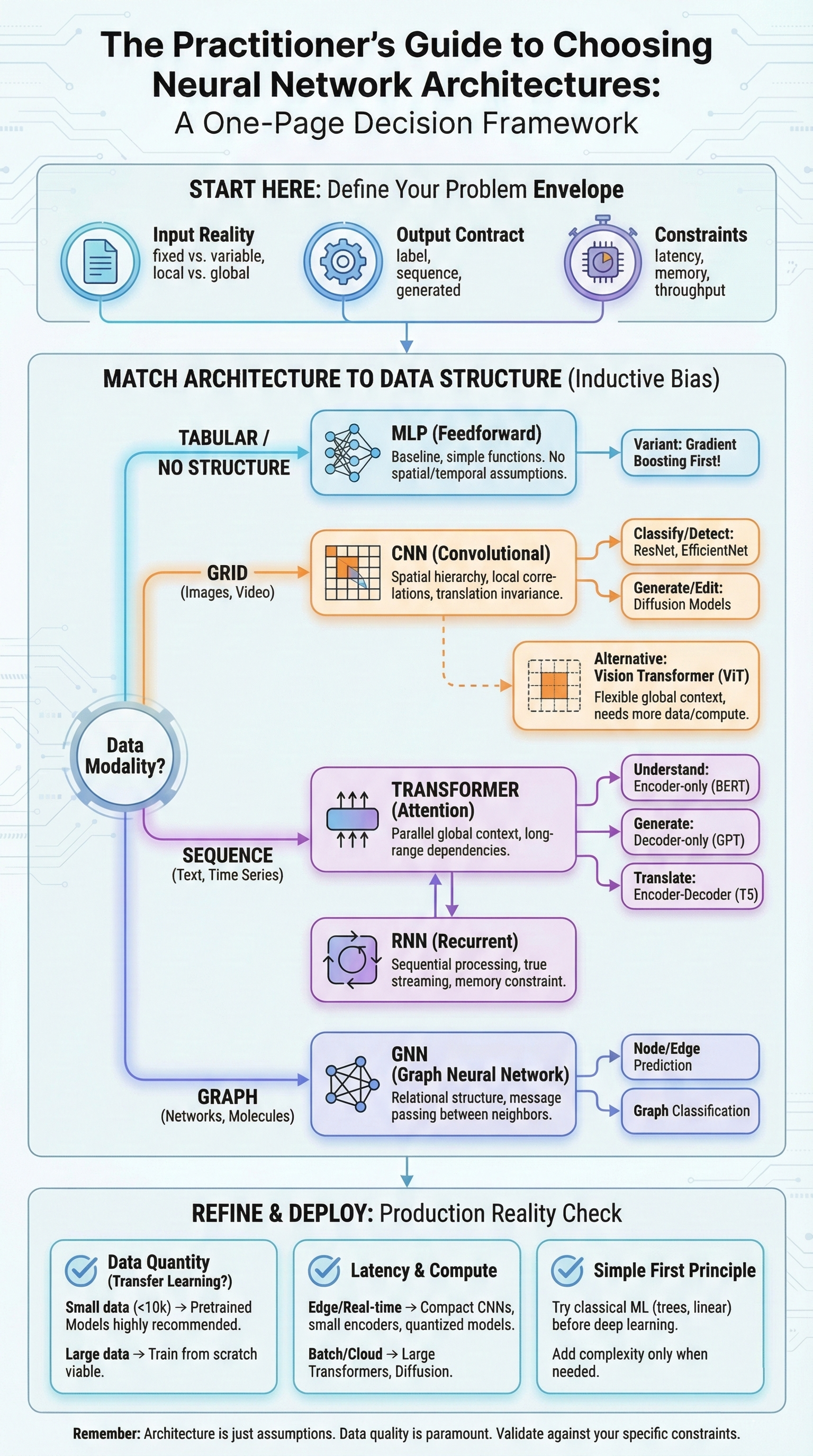
Figure 0: One-Page Decision Framework - From problem definition to architecture selection
Picture this. You're staring at a new machine learning project with data spread across your desk—images, text, time series, transactions, maybe all of the above. Neural networks can probably help. But which one?
A quick search reveals hundreds of architectures. ResNet, BERT, GPT, LSTMs, GNNs, diffusion models, Vision Transformers, and countless variants flood your screen. Each paper claims state-of-the-art results. Each tutorial assumes you already know which model fits your problem. Nobody tells you how to decide.
This guide fixes that problem.
You'll learn to match architectures to data characteristics, understand the tradeoffs that matter in production, and avoid the expensive mistakes that derail ML projects. No hype here. No "Transformers for everything." No solutions searching for problems. Just practical guidance for practitioners who need to ship working systems.
Table of Contents
- Before You Read Further: The Model Brief
- Part 1: Foundational Concepts
- Part 2: Taxonomy Framework
- Part 3: Architecture Deep-Dives
- Part 4: Choosing Variants Within Families
- Part 5: The Decision Framework
- Part 6: Common Pitfalls
- Part 7: Data, Objectives, and Evaluation
- Part 8: Production and Deployment
- Part 9: Quick Reference Materials
- Final Principles
- Appendix: Training Mechanics
Before You Read Further: The Model Brief
Before comparing architectures, answer these questions. If you can't, you'll end up choosing by hype instead of fit.
Input Reality
- What's the true input form at inference? (single image vs video clip; one document vs stream; full graph vs local neighborhood)
- Are inputs fixed-size or variable-length?
- Is the signal local (nearby pixels/events matter most) or global (distant relationships matter)?
Output Contract
- Single label, multiple labels, structured fields, sequence, mask, ranked list, or generated content?
- Do you need calibrated confidence or just an argmax?
Constraint Envelope
- Latency: realtime (<10ms) vs near-realtime vs batch
- Memory: edge/mobile vs server
- Throughput: occasional requests vs high QPS
Risk/Governance
- Explainability requirements?
- Safety tolerance (false negatives vs false positives)?
Keep this brief in mind as you read. Every architecture recommendation traces back to these constraints.
Part 1: Foundational Concepts
These concepts determine why one architecture succeeds where another fails. If you already work with neural networks daily, skim to "Why Architecture Matters"—that's the core insight.
What Neural Networks Actually Do
Neural networks are function approximators. They learn to map inputs to outputs by discovering patterns in data—transformation pipelines where raw data enters one end and predictions emerge from the other.
The key insight is representation learning. A neural network doesn't just memorize input-output pairs. It discovers intermediate representations that make the mapping easier. When classifying images, early layers detect edges and textures. Middle layers combine these into parts and shapes. Final layers recognize objects. The network learns a hierarchy of increasingly abstract features.
Why does this matter? Different architectures make different assumptions about what representations will be useful. Match your architecture's assumptions to your data's actual structure, and learning becomes dramatically easier.
The Training Loop (Compressed)
Training is iterative optimization. Four steps repeat: (1) Forward pass—data flows through, network produces prediction. (2) Loss calculation—measure how wrong the prediction was. (3) Backpropagation—compute how each parameter contributed to error. (4) Optimization—adjust parameters to reduce loss.
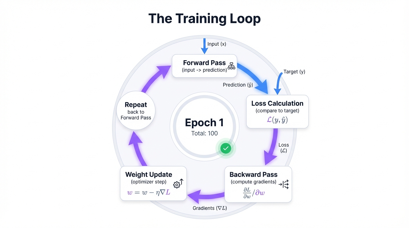
This loop repeats thousands or millions of times. Each iteration nudges the network toward better predictions. For deeper coverage, see Appendix: Training Mechanics.
Key Distinctions
Parameters are values the network learns (weights and biases). Hyperparameters are choices you make before training (learning rate, architecture, layer count). Architecture selection is a hyperparameter decision—you're choosing structural constraints within which learning occurs.
Overfitting means the model memorizes training data instead of learning generalizable patterns. Underfitting means the model is too simple to capture the signal. Architecture choice directly influences this tradeoff—you're choosing structural constraints that guide how the network learns.
Why Architecture Matters: Inductive Bias
Here's the insight that motivates this entire guide. Architecture isn't just a technical detail. It's a set of assumptions about your data encoded in mathematical structure.
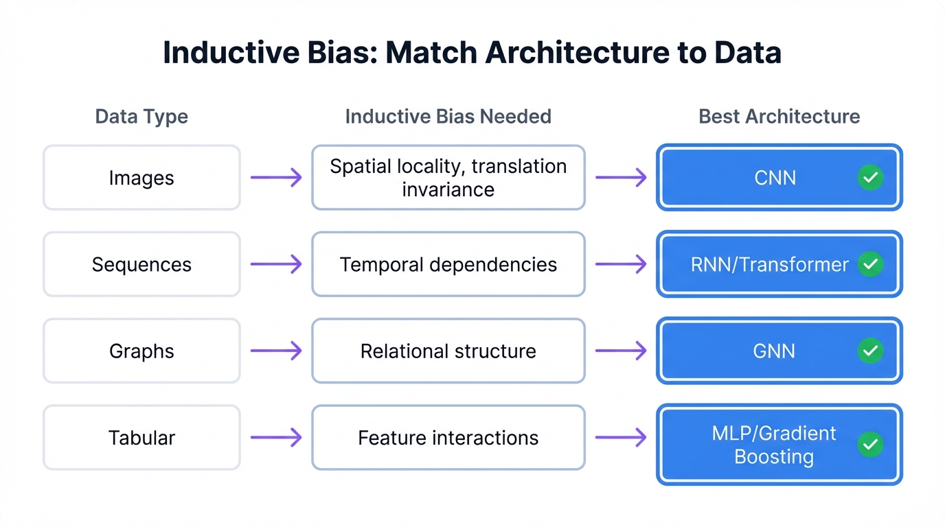
This is called inductive bias—the assumptions a model makes about data to learn effectively.
- CNNs assume nearby pixels correlate more strongly than distant ones
- RNNs assume earlier elements in a sequence influence later ones
- Transformers assume any element might relate to any other, but let data determine which relationships matter
- GNNs assume your data has explicit relational structure
- MLPs encode minimal structure compared to other families—everything is potentially related to everything
When your architecture's assumptions match your data's true structure, learning becomes dramatically more efficient. The network doesn't have to discover from scratch that adjacent pixels matter. Convolution embeds that knowledge. When assumptions mismatch, the network either fails to learn or requires vastly more data to overcome the architectural bias.
Key Insight: Architecture selection, then, is fundamentally about matching structural assumptions to your data's characteristics.
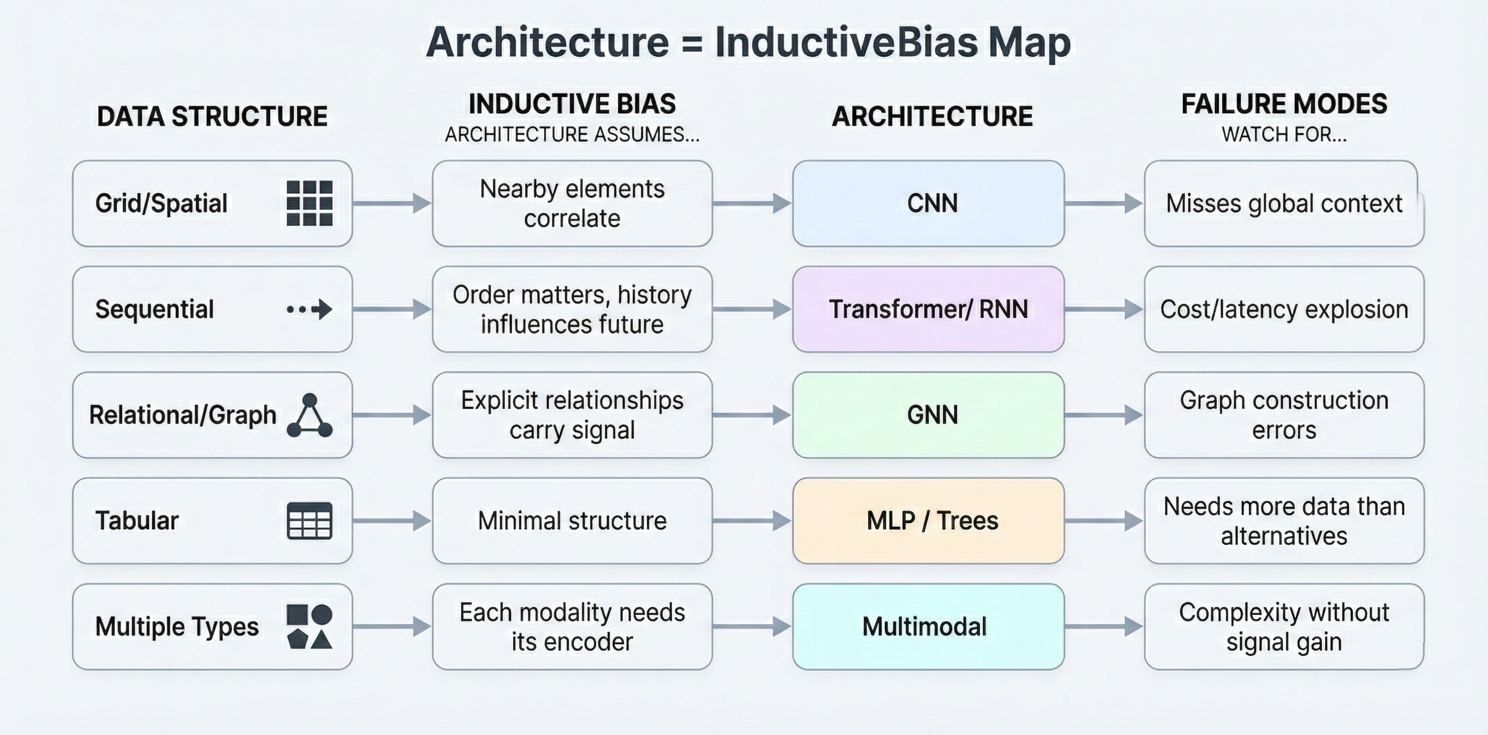
Figure 1: Architecture = Inductive Bias - Matching data structure to the right architecture
Failure Mode Mapping
When your model underperforms, the architecture often points to why:
| Family | Typical Failure Mode | Symptom |
|---|---|---|
| CNN | Misses global context | Fails on relationships between distant image regions |
| Transformer | Cost/latency explosion | Works but too slow or expensive for production |
| RNN/LSTM | Long-range forgetting | Accuracy degrades on longer sequences |
| GNN | Graph construction errors | Model learns noise in edge definitions |
| MLP | No structure exploitation | Needs vastly more data than structured alternatives |
Use this table to diagnose problems, then consider variant changes or family switches.
Part 2: Taxonomy Framework
Three distinct dimensions characterize any machine learning approach: architecture families, learning paradigms, and task domains. Understanding how these intersect prevents the common confusion of conflating structure with training method with objective.
Architecture Families (The Structure)
Architecture families define how data flows through a network and how layers connect. They're structural blueprints, independent of what task you're solving or how you're training.
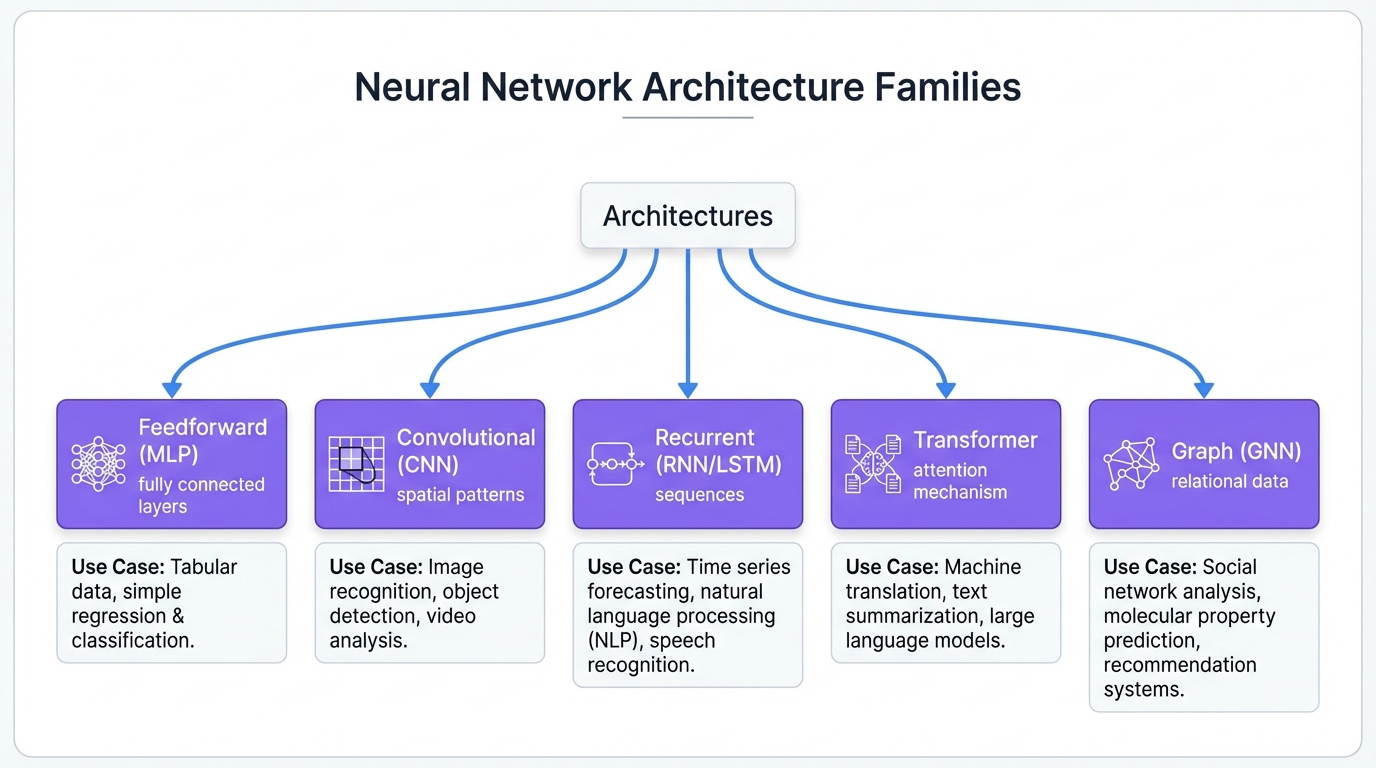
| Family | Core Principle | Data Flow |
|---|---|---|
| Feedforward (MLP) | Sequential layers, no cycles | Input → Hidden → Output |
| Convolutional (CNN) | Local connectivity via sliding filters | Hierarchical feature extraction |
| Recurrent (RNN) | Connections form cycles; state persists | Sequential with memory |
| Transformer | Attention relates all positions | Parallel with learned relevance |
| Graph (GNN) | Message passing between nodes | Structure-aware aggregation |
Learning Paradigms (How It Learns)
Learning paradigms describe the relationship between model and training signal. They're orthogonal to architecture—any family can train under different paradigms.
Supervised Learning: Learn from labeled input-output pairs. Most common when labeled data is available.
Unsupervised Learning: Discover structure without labels—clusters, distributions, compressed representations.
Self-Supervised Learning: Create supervision from data itself. Mask part of an input and predict the masked portion. Learn rich representations without human-provided labels, then transfer to downstream tasks.
Reinforcement Learning: Learn from interaction with an environment. Actions produce rewards and state changes. Suits sequential decision-making.
Task Domains (What You Want)
What output do you need from what input?
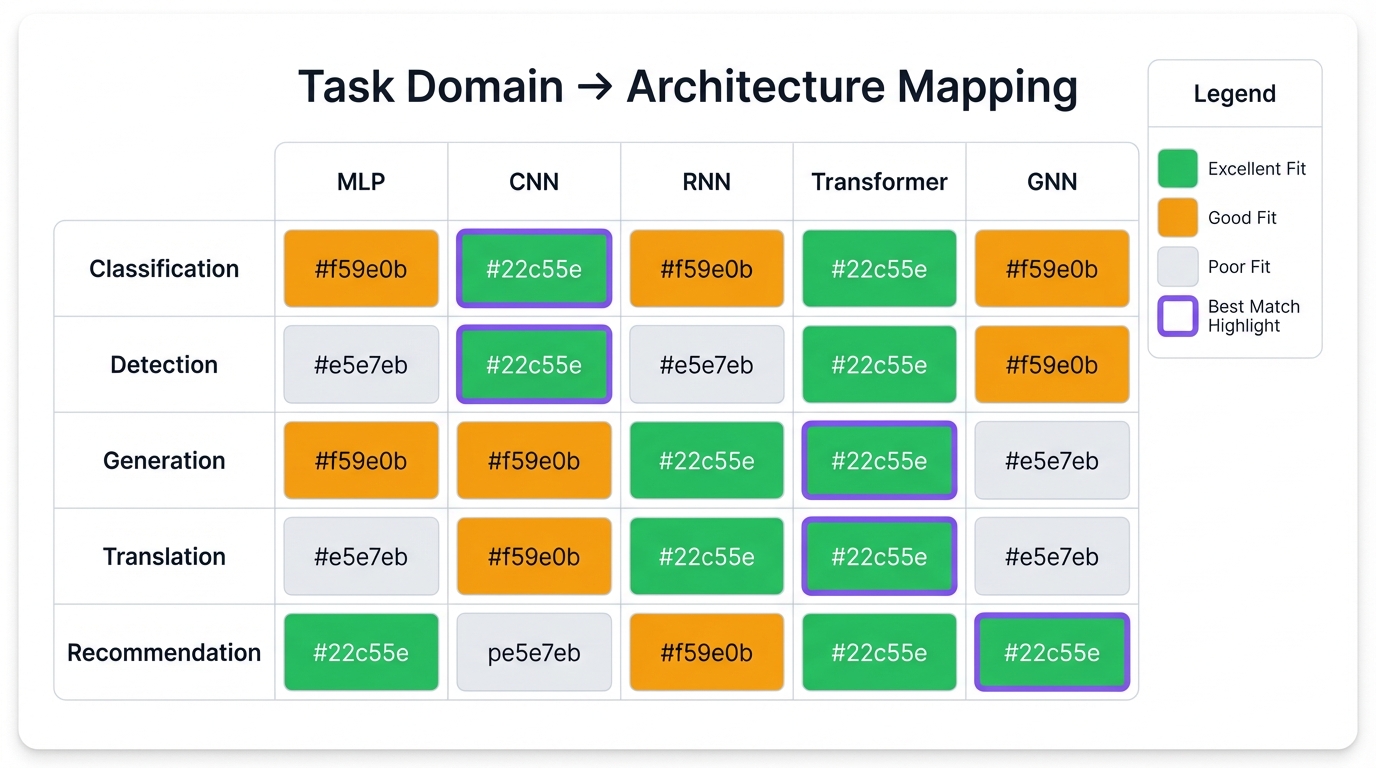
| Task | Input → Output | Examples |
|---|---|---|
| Classification | Data → Category | Spam detection, defect identification |
| Regression | Data → Continuous value | Price prediction, forecasting |
| Generation | Condition → New data | Image synthesis, text completion |
| Detection | Scene → Located objects | Autonomous vehicles, security |
| Segmentation | Image → Pixel labels | Medical imaging, satellite analysis |
| Translation | Sequence → Sequence | Language translation, summarization |
How They Intersect
These dimensions combine independently. A Transformer (architecture) trained with self-supervision (paradigm) for text generation (task). The same Transformer, trained with supervision, might perform classification instead.
The key insight: architecture selection flows primarily from data characteristics, not from paradigm or task alone.
Ask: What structure does my data have? Images have spatial structure; sequences have temporal structure; social networks have graph structure. Match your architecture to that structure.
Then ask: What's my task? This influences architecture details and output design, but the core family was already suggested by data structure.
Finally ask: What paradigm fits my supervision situation? This affects training procedures but rarely changes fundamental architecture choice.
Part 3: Architecture Deep-Dives
Now we examine each major architecture family. For each: the motivating insight, core mechanism, ideal use cases, honest tradeoffs, and clear signals you should look elsewhere.
3.1 Feedforward Networks (MLPs): The Baseline That Wins More Than People Admit
The Motivating Insight
If single-layer networks can only learn linear boundaries, what happens when you stack layers? The answer, proved by the universal approximation theorem, is that sufficiently wide networks with nonlinear activations can approximate any continuous function. MLPs are the foundation upon which all other architectures build.
Core Mechanism
An MLP passes data through sequential fully-connected layers. Each layer performs a linear transformation (matrix multiply plus bias) followed by a nonlinear activation. "Fully connected" means every neuron in one layer connects to every neuron in the next. There's no special structure, no assumptions about spatial or temporal relationships.
Think of it as coordinate transformations. Each layer warps the data space, and nonlinear activation allows nonlinear warping. Stack enough layers, and you can sculpt the space to separate any pattern.
Ideal Use Cases
- Tabular data (spreadsheets, structured logs, business metrics)
- Feature vectors from other systems
- Classification heads on top of other architectures
- Any data lacking obvious spatial/temporal structure
Strengths
- Simple mental model, easy to deploy
- Often strong with good feature engineering
- Fast iteration, predictable behavior
- Efficient inference, small memory footprint
Limitations
- No structural assumptions means no free lunch—can't exploit known patterns
- Processing images requires flattening, losing spatial relationships
- Must learn from scratch that adjacent pixels relate, dramatically increasing data requirements
- Parameter count scales quadratically with width
When to Skip: Raw images, text, audio, or any data where structure matters. Using an MLP here isn't wrong, but you're handicapping yourself unnecessarily.
3.2 Convolutional Neural Networks (CNNs): Spatial Hierarchy
The Motivating Insight
Images have spatial structure. Pixels near each other tend to represent the same object. The same pattern (an edge, a face) should be recognized regardless of where it appears. CNNs encode these insights directly.
Core Mechanism
The fundamental operation is convolution: sliding a small filter across the input and computing the dot product at each position. A filter is a learned pattern detector. An edge-detecting filter produces high activations where edges align with its pattern. A CNN learns many filters per layer, each detecting different patterns.
Pooling operations provide translation invariance and reduce spatial dimensions. A feature detected anywhere in a local region is reported; exact position doesn't matter.
Stacking layers creates a feature hierarchy. Early layers detect edges and colors. Middle layers combine these into textures and parts. Deep layers detect objects and scenes. The receptive field—input region influencing each output—grows with depth.
Ideal Use Cases
- Image classification, detection, segmentation
- Medical imaging analysis
- Satellite imagery
- Audio spectrograms
- Any data with grid-like topology and local correlations
Key Variants
- ResNet: Residual connections enable very deep networks
- EfficientNet: Systematic scaling of depth/width/resolution
- ConvNeXt: Modern CNN matching Transformer performance
Strengths
- Parameter efficiency through weight sharing
- Strong inductive bias for spatial data
- Excellent performance with limited data
- Fast inference, highly optimized
Limitations
- Fixed receptive field constraint—global dependencies require many layers
- Struggles without grid structure
- Position information can be lost when it matters
When to Skip: Data lacking grid structure or spatial locality. Text suits sequence models. Graphs need graph networks. Tabular data suits MLPs or gradient boosting.
3.3 Recurrent Networks (RNNs/LSTMs/GRUs): Sequential Memory
The Motivating Insight
Sequences have temporal structure. The meaning of a word depends on preceding words. Predicting the next sensor reading depends on recent history. RNNs encode sequential dependencies through cycles in the network graph.
Core Mechanism
At each timestep, an RNN takes current input and previous hidden state, combines them through a learned transformation, and produces a new hidden state plus output. The hidden state is memory—a compressed representation of the sequence so far.
Vanilla RNNs struggle with long sequences due to vanishing gradients. LSTMs and GRUs address this through gating mechanisms that control information flow, allowing gradients to flow over longer distances.
Status Today
Often replaced by Transformers, temporal convolutions (TCNs), or state-space models (SSMs like Mamba) for most tasks—but not dead. RNNs retain advantages in:
- Very long sequences where attention's quadratic cost becomes prohibitive
- True streaming/online processing with minimal latency
- Edge deployment with tight memory constraints
- Simple sequence tasks where data is scarce
Strengths
- Natural variable-length sequence handling
- Constant memory regardless of sequence length
- True online processing capability
- Parameter efficient for sequential data
Limitations
- Sequential processing prevents parallelization—slow training
- Even LSTMs struggle with very long dependencies
- Fixed-size hidden state creates information bottleneck
- Transformers have proven more effective when compute allows
When to Skip: Most language tasks, most sequence classification, and most generation tasks where sequences fit in memory. Transformers usually dominate here when compute allows. Consider RNNs when sequence length is extreme, memory is constrained, or you need true streaming.
3.4 Transformers: The Attention Engine
The Motivating Insight
What if you didn't need to process sequences sequentially? RNNs' sequential nature limits parallelization and creates bottlenecks. What if every position could directly attend to every other position?
Core Mechanism
Self-attention works through three projections: queries, keys, and values. Each position produces a query ("what am I looking for?"), a key ("what do I contain?"), and a value ("what should I contribute if selected?"). Attention weights come from comparing queries to keys; outputs come from weighted sums of values.
Think of it as a differentiable dictionary lookup. Queries search for relevant keys, and attention weights determine how much each value contributes. The lookup is soft (weighted combinations) rather than hard (single selection), making it trainable.
Multi-head attention runs multiple attention operations in parallel. Different heads capture different relationship types: syntax, semantics, positional patterns.
Architectural Variants
| Variant | Attention Type | Best For |
|---|---|---|
| Encoder-only (BERT) | Bidirectional | Understanding, classification, extraction |
| Decoder-only (GPT) | Causal (past only) | Generation, completion |
| Encoder-decoder (T5) | Cross-attention | Translation, summarization |
Ideal Use Cases
- All text tasks: classification, generation, translation, summarization
- Code generation and understanding
- Vision (with patches): ViT, when data/compute allows
- Audio, video, proteins, molecules
- Any domain requiring flexible global context
Strengths
- Parallel processing across positions
- Direct long-range dependency modeling
- Flexible learned attention patterns
- Massive scalability with data and compute
- Pretraining + fine-tuning is a practical superpower
Limitations
- Quadratic complexity in sequence length—doubling length quadruples compute
- Lack strong inductive biases—need substantial data
- Memory requirements during training can be substantial
- Autoregressive inference is sequential
When to Skip: Small tabular problems where trees dominate. Tight latency/compute budgets without pretrained options. Vision tasks with limited data where CNN transfer learning is simpler.
3.5 Graph Neural Networks (GNNs): Learning on Relationships
The Motivating Insight
Standard architectures assume data fits in a grid (images) or a line (text). What if your data is a social network, a molecule, or a supply chain? Forcing graph data into grids loses the relational structure that contains the signal.
Core Mechanism
Message passing: nodes aggregate information from neighbors to update their representations. After several rounds, each node encodes multi-hop context about its local neighborhood.
Think of it as iterative neighborhood polling. Each round, nodes ask their neighbors "what do you know?" and combine those answers with their own state. After K rounds, each node's representation reflects information from nodes up to K hops away.
Ideal Use Cases
- Fraud detection on transaction networks
- Recommendation systems (user-item graphs)
- Molecular property prediction (atoms as nodes, bonds as edges)
- Social network analysis
- Knowledge graph reasoning
- Supply chain optimization
Strengths
- Strong inductive bias for relational structure
- Generalizes across graph sizes and topologies
- Supports node, edge, and graph-level predictions
- Natural handling of irregular structure
Limitations
- Scaling to huge graphs is challenging
- Oversmoothing limits depth
- Graph construction quality matters enormously
- Long-range propagation can be difficult
Key Considerations
| Graph Type | Implication |
|---|---|
| Homogeneous (one node/edge type) | Standard GNN approaches |
| Heterogeneous (multiple types) | Need type-aware architectures |
| Static | Standard training |
| Dynamic (edges change) | Time-aware modeling required |
| Transductive (predict on training nodes) | Easier |
| Inductive (generalize to new nodes) | More realistic for production |
When to Skip: If relationships are weak proxies or noise. If your "graph" is just a workaround for missing feature engineering. A simpler tabular model over engineered relational features may beat a fancy GNN with poorly constructed edges.
3.6 Generative Architectures: Creating, Not Classifying
Generative modeling learns a distribution so you can sample, synthesize, or impute.
VAEs (Variational Autoencoders)
Intuition: Learn a compressed latent space that can generate plausible samples.
Strengths: Stable training, useful latent representations, good for anomaly detection via reconstruction.
Limitations: Samples can be blurry compared to newer approaches.
Use when: You need representation learning, anomaly detection, or controllable generation with smooth interpolation.
GANs (Generative Adversarial Networks)
Intuition: Generator creates samples, discriminator judges realism—they compete.
Strengths: Sharp, realistic samples in specialized settings.
Limitations: Training instability, mode collapse, tricky evaluation.
Use when: Specialized image synthesis where sharpness matters and you can manage training complexity.
Diffusion Models
Intuition: Learn to reverse a gradual noising process—turn noise into structure step-by-step.
Strengths: High-quality generation, excellent controllability, state-of-the-art for images.
Limitations: Multi-step sampling is slower (though acceleration methods exist).
Use when: Modern image generation/editing, high-fidelity synthesis, conditional generation. This is the current default for image generation.
When to Skip Generative Altogether: If your "generation" is actually classification or retrieval in disguise. If you only need a decision, not a novel artifact, start with discriminative models.
3.7 Hybrid and Multimodal Architectures
Real problems often involve multiple data types: images + text, audio + metadata, logs + topology.
Vision Transformers (ViT)
Transformers applied to image patches. Competitive especially with large-scale pretraining. Consider when you have abundant data or strong pretrained models available.
CLIP-Style Models
Align images and text into shared embedding space. Excellent for zero-shot classification, retrieval, and "find images matching this description" workflows.
Cross-Modal Fusion Strategies
| Strategy | Mechanism | Best For |
|---|---|---|
| Dual-encoder | Separate encoders, shared embedding space | Retrieval, fast matching |
| Cross-attention | One modality attends to another | Deep grounding, VQA |
| Late fusion | Combine features near output | Loosely coupled modalities |
When to Skip: Single-modality tasks with limited data and strict latency. When a strong unimodal baseline already meets requirements. Adding modalities without clear signal improvement just adds complexity.
Part 4: Choosing Variants Within Families
Selecting the architecture family is step one. Step two is choosing the right variant within that family. Use the Model Brief you filled out at the start as your filter for these decisions.
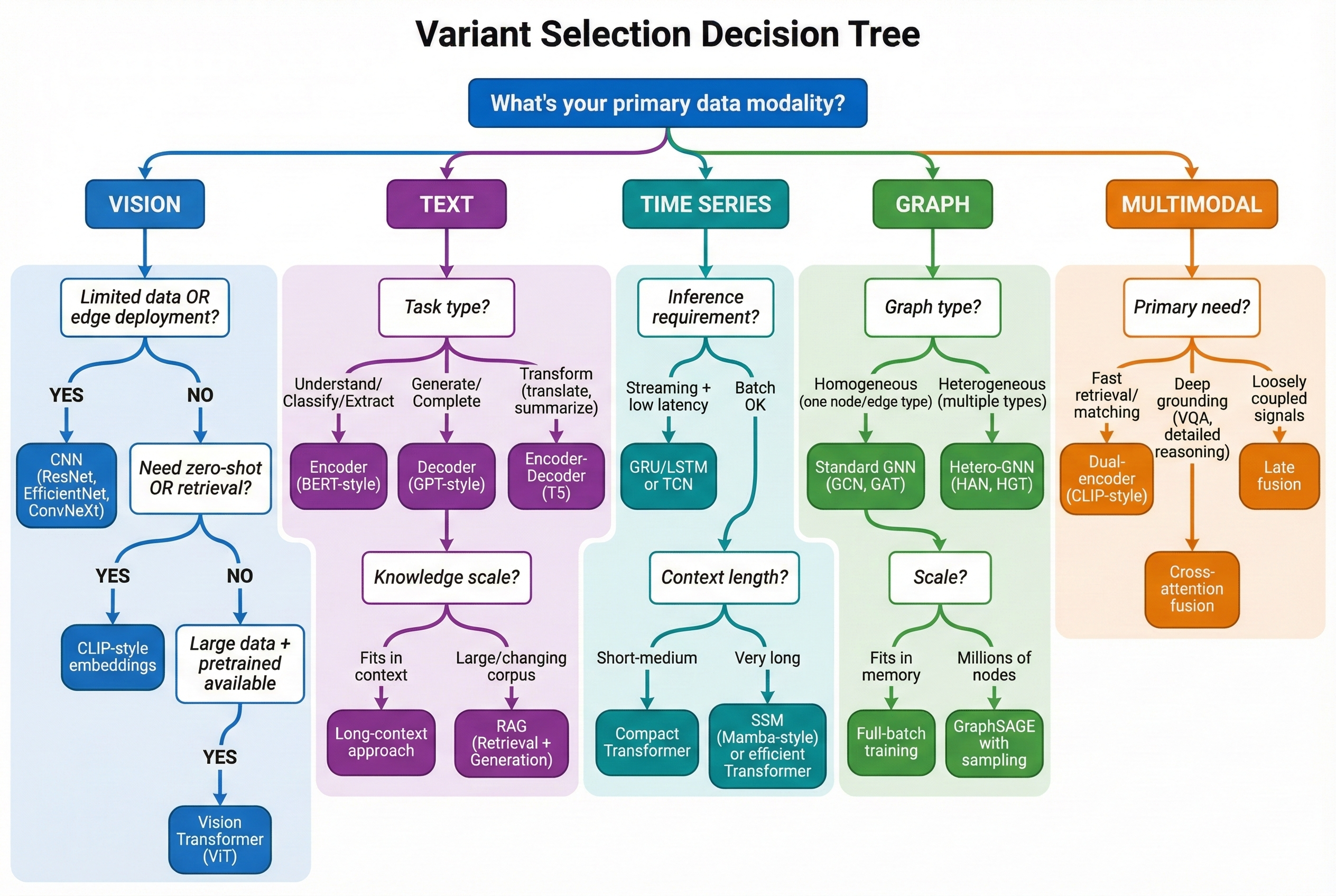
Figure 2: Variant Selection Decision Tree - Navigate from your data modality to the right architecture variant
Vision Variants: CNN vs ViT vs Embeddings-First
Within vision, you're choosing between three strategies:
CNN Family (ResNet/EfficientNet/ConvNeXt)
- Pick when: strong performance with limited data, predictable latency, edge deployment, classic detection/segmentation
- ResNet: dependable, strong baseline, easy to reason about
- EfficientNet: care about accuracy-per-compute, scaling sensibly
- ConvNeXt: modernized CNN narrowing gap with Transformer-era designs
Vision Transformers (ViT)
- Pick when: you can leverage strong pretrained backbones or have abundant data; want flexible global interactions
- Skip when: compute/latency constrained or data-limited without pretrained options
Embeddings-First (CLIP-style)
- Pick when: fast iteration, retrieval, similarity search, zero-shot or few-shot classification
- Key question: Is your task recognition or matching? If matching, embeddings often win.
- Skip when: need pixel-level outputs (segmentation) or fine-grained detection
Concrete Examples:
- Circuit board defect detection: consistent, low-latency classification on inspection line → CNN variants first
- "Find visually similar defects across factories" → embeddings-first approach
Text Variants: Encoder vs Decoder vs Encoder-Decoder
The most important variant choice in NLP isn't model name—it's interaction style.
Encoder-Only (BERT-style)
- Pick when: task is understanding (classification, extraction, tagging, search re-ranking)
- Why: strong representation of entire input at once
- Skip when: need multi-step generation or long-form outputs
Decoder-Only (GPT-style)
- Pick when: task is generation (drafting, completion, multi-turn interaction, code synthesis)
- Tradeoff: generation is inherently sequential; "smart + fast" is harder
- Skip when: only need classification/extraction—encoders are more efficient
Encoder-Decoder (T5-style)
- Pick when: input → output is a transformation (translation, summarization, structured rewriting)
- Why: naturally models "read fully, then produce"
Long-Context vs Retrieval
A major architecture-level fork:
- Long-context-first: put entire relevant world in context window. Pick when info is reliably small or need tightly coupled reasoning.
- Retrieval-first (embed + fetch + read): represent documents as embeddings, retrieve candidates, then read. Pick when knowledge base is large, changes frequently, or need auditability.
Time Series Variants: Streaming vs Global Context
Streaming-Friendly
- Pick when: must process events online, keep latency minimal, don't need huge context
- Aligns with recurrent-style or temporal convolution approaches
Global-Context
- Pick when: long-range dependencies matter (slow-burn anomalies, periodicity, multi-stage incidents)
- Transformer-style sequence models are the match
Practical Rule: If you can't afford to "look back" far at inference time, don't pick an architecture that only shines with long context.
Graph Variants: Match the Graph's Nature
Most GNN failures are graph-definition failures. Variant selection starts with understanding the graph.
Homogeneous vs Heterogeneous
- Homogeneous: one node/edge type (simpler)
- Heterogeneous: many entity types and relation types (fraud, security, enterprise data)
- Pick hetero-capable approaches when type matters
Static vs Dynamic
- Static: relationships don't change often (molecules, knowledge graphs)
- Dynamic: edges appear/disappear (transactions, network flows)
- Dynamic settings need time-aware designs
Transductive vs Inductive
- Transductive: predict on nodes seen during training
- Inductive: generalize to new nodes/graphs
- Production usually needs inductive behavior
Generation Variants: Pick by Output Requirements
Diffusion
- Pick when: high-fidelity images and edits matter most; controllability valuable
- Skip when: ultra-low-latency without multi-step sampling
Autoregressive (Transformer Decoders)
- Pick when: generating tokens (text/code) or structured sequences
- Skip when: primarily need image synthesis
VAE
- Pick when: smooth latent space for representation, interpolation, anomaly detection
- Skip when: want best-possible visual realism
GAN
- Pick when: specialized image synthesis niche, can tolerate complexity
- Skip when: stability and predictability matter more than peak sharpness
Multimodal Variants: Three Fusion Patterns
Dual-Encoder (CLIP-style)
- Separate encoders, shared embedding space
- Pick when: retrieval/matching, fast zero-shot classification
- Strength: scalable, fast at inference
Cross-Encoder / Cross-Attention
- One modality attends to another directly
- Pick when: deep grounding needed ("this word refers to that region"), VQA
- Cost: heavier and slower
Late Fusion
- Combine features near the end
- Pick when: modalities are loosely coupled (image + metadata + tabular)
- Often the simplest strategy that works
Part 5: The Decision Framework
Data Quantity Thresholds
These aren't hard rules—use them as starting instincts:
| Data Size | What You Can Realistically Do |
|---|---|
| < 1,000 samples | Classical ML (trees, linear). Heavy transfer learning if using neural nets. |
| 1,000-10,000 | Transfer learning essential. Fine-tune pretrained models. |
| 10,000-100,000 | Most architectures viable with pretrained starting points. |
| 100,000+ | Training larger models from scratch becomes reasonable. |
The thresholds shift dramatically with transfer learning. A pretrained vision model can perform well with hundreds of labeled images. Training from scratch requires orders of magnitude more.
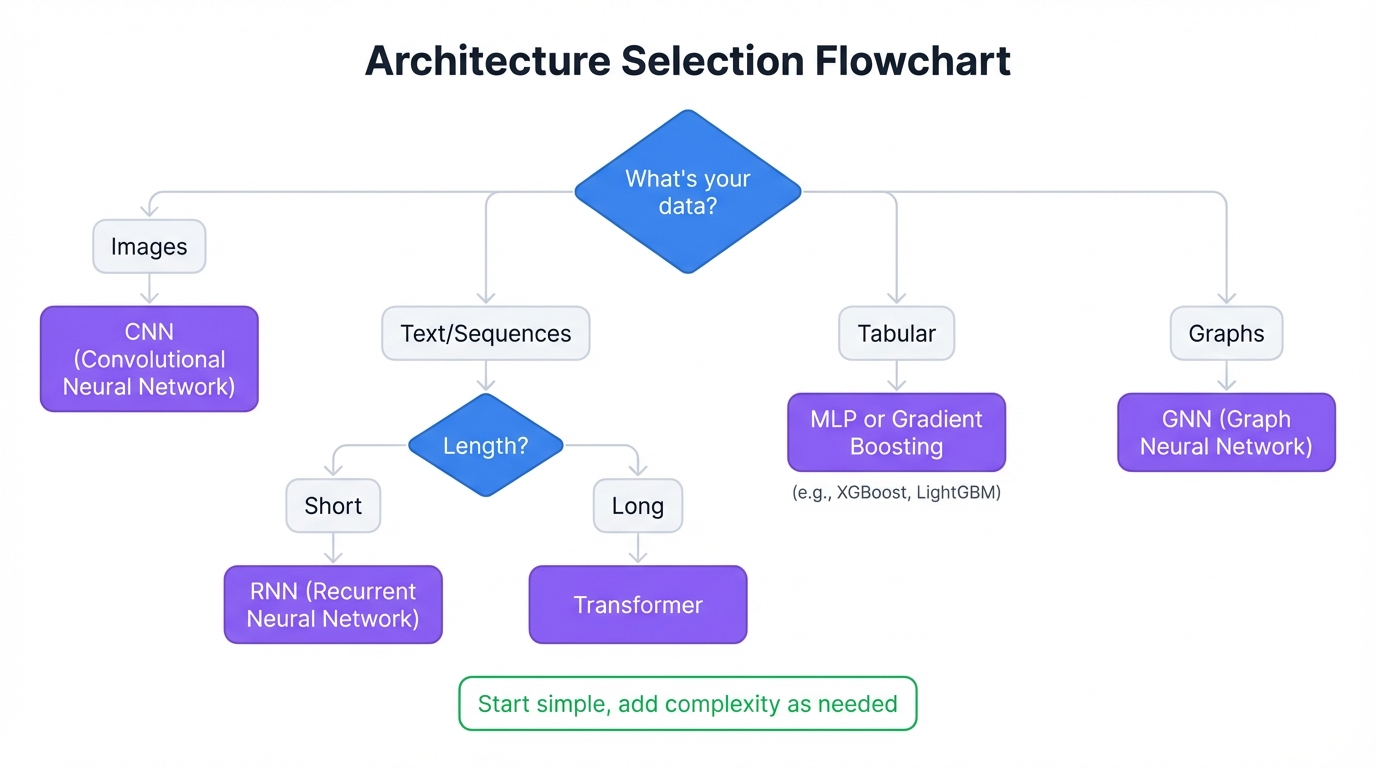
Primary Decision Flow
Start with your data modality:
TABULAR DATA (rows/columns, business metrics)
├── Need prediction (classification/regression)?
│   └── Start: Gradient boosting / linear models
│       └── If needed: MLP as next step
└── Need generation/imputation?
    └── VAE-like approaches (niche)

IMAGES / VIDEO (grids)
├── Classification / detection / segmentation?
│   ├── Limited data or edge constraints → CNN (ResNet/EfficientNet/ConvNeXt)
│   └── Large data / want pretrained reps → ViT / CLIP-style
└── Image generation/editing
    └── Diffusion (modern default), GAN (specialized)

TEXT / CODE (token sequences)
├── Understand/classify/extract → Transformer encoder (BERT-style)
├── Generate/continue → Transformer decoder (GPT-style)
└── Translate/transform → Encoder-decoder (T5-style)

TIME SERIES / EVENT SEQUENCES
├── Short context / streaming / tiny budget → GRU/LSTM or temporal CNN
└── Long context / rich dependencies → Transformer

GRAPHS (entities + relations)
├── Node/edge/graph prediction → GNN (message passing)
└── Very large / long-range → Scalable GNN or graph-transformer hybrid
Constraint-Based Filtering
After identifying candidate architectures, filter by real-world constraints:
Latency Requirements
- Real-time / edge (<10ms): CNNs for vision, small encoders for NLP, compact MLPs, small GRUs
- Batch processing: Heavier Transformers, diffusion, bigger GNNs are acceptable
Training Data Volume
- Thousands of samples: Strong inductive bias + transfer learning (CNNs, pretrained encoders)
- Millions+: Transformers/ViTs from scratch become reasonable
Compute Budget
- Laptop / modest GPU: MLPs, compact CNNs, pretrained encoders, small Transformers
- Cloud cluster: Large Transformers, multimodal, bigger diffusion, large graphs
Interpretability
- If stakeholders require explanations, start simpler or use architectures with interpretable components
Deployment Target
- Mobile/edge/browser: Memory + latency dominate → compact CNNs/MLPs, distilled models
- Server: Trade hardware for accuracy
The "Simple First" Principle
In practice, this wins most projects:
- Start with the simplest architecture matching your data structure
- Only add complexity when you can point to a specific gap:
- "Model misses global context" → consider attention/Transformers
- "Model struggles with spatial patterns" → consider CNN/ViT
- "Signal is relational" → consider GNN
- "Need generation" → diffusion/GAN/VAE
Key Principle: Complexity should be a response to evidence, not fashion.
Where Newer Techniques Fit
You may encounter these terms and wonder where they belong:
RAG (Retrieval-Augmented Generation): Not an architecture—a pattern combining retrieval with generation. Uses embeddings for search + Transformer for reading/generating. Already covered under "Long-Context vs Retrieval" in text variants.
Mixture-of-Experts (MoE): A scaling strategy for Transformers. Routes inputs to specialized sub-networks, giving higher capacity without proportional inference cost. Consider when you need very large models but want manageable serving costs.
State-Space Models (SSMs)—like Mamba: Sequence models optimized for very long contexts and streaming. Competitive with Transformers on some benchmarks while being more efficient on long sequences. Consider when sequence length exceeds practical Transformer limits.
Tabular Deep Learning (FT-Transformer, TabNet): Neural approaches specifically designed for tabular data. Can beat gradient boosting in some cases, but the "GBDT first" principle still holds—try trees before reaching for these.
These don't change the core framework. They're refinements within families you already understand.
Quick Decision Reference
| If You Have | And Need | Consider First |
|---|---|---|
| Circuit board images | Defect classification | CNN (ResNet/EfficientNet) |
| Customer churn table | Classification | Gradient boosting → MLP if justified |
| Long documents | Classification/extraction | Transformer encoder |
| Code completion | Generation | Transformer decoder |
| Security logs | Anomaly detection | Sequence Transformer or compact RNN |
| Transaction network | Fraud detection | GNN |
| Molecular structures | Property prediction | GNN |
| Image synthesis | Generation/editing | Diffusion |
| Text + images | Joint understanding | CLIP / multimodal Transformer |
Worked Examples: Five Real Decisions
1. Vision: Manufacturing Defect Detection
Problem: Detect surface defects on machined parts from inspection camera images.
Input reality: Single high-res images, ~50k labeled examples, need <100ms inference on factory edge device.
Constraints: Edge deployment (limited GPU), must handle new defect types quarterly.
Pick: CNN (EfficientNet-B0 or MobileNetV3) with transfer learning from ImageNet.
Why not ViT: Data volume is moderate, edge constraints favor CNN efficiency.
Why not CLIP: Need detection/localization, not just classification.
2. Text: Customer Support Ticket Routing
Problem: Classify incoming support tickets into 15 categories for team routing.
Input reality: Short text (50-200 words), 200k labeled tickets, batch processing acceptable.
Constraints: Accuracy matters more than latency. Need to add new categories occasionally.
Pick: Transformer encoder (fine-tuned DistilBERT or similar).
Why not GPT-style: Classification doesn't need generation capability.
Why not classical ML: Text semantics benefit from pretrained representations.
3. Time Series: Account Takeover Detection
Problem: Detect account takeover from authentication event logs.
Input reality: Streaming events, need to flag within 500ms of suspicious pattern, long-tail anomalies matter.
Constraints: Low latency, must handle bursty traffic, retrain weekly.
Pick: Compact Transformer or GRU baseline—start with GRU for latency, upgrade if accuracy insufficient.
Why not large Transformer: Latency constraint; streaming inference favors recurrent-style.
Why not CNN: Temporal dependencies matter more than local patterns.
4. Graph: Fraud Ring Detection
Problem: Identify coordinated fraud networks from transaction relationships.
Input reality: Heterogeneous graph (users, accounts, devices, merchants), dynamic edges, millions of nodes.
Constraints: Daily batch scoring, need inductive capability for new accounts.
Pick: GNN with GraphSAGE-style sampling for scalability, heterogeneous message passing.
Why not tabular: Relational structure is the signal—isolated features miss coordination patterns.
Why not Transformer: Graph structure is explicit; attention alone doesn't encode topology.
5. Multimodal: Product Search with Images and Text
Problem: Enable "find products like this" from user-uploaded photos plus text queries.
Input reality: Image + optional text query, need to rank from 10M product catalog.
Constraints: <200ms retrieval, catalog updates daily, zero-shot generalization to new products.
Pick: CLIP-style dual encoder (image + text → shared embedding space) with approximate nearest neighbor search.
Why not cross-attention: Retrieval over 10M items requires fast embedding comparison, not pairwise scoring.
Why not fine-tuned CNN: Zero-shot requirement favors pretrained multimodal embeddings.
Part 6: Common Pitfalls
"Transformers Are Always Best"
They're often best when pretrained representations matter and global context is needed. But they can be wasteful for:
- Small tabular problems
- Simple vision with limited data
- Strict edge constraints
Overengineering: Sledgehammer for a Nail
Signals you're overbuilding:
- Your dataset is small and you're reaching for the heaviest architecture
- You can't articulate what relationship structure simpler models can't capture
- You're adding modalities "because it might help"
Underestimating Classical ML on Tabular
Tree ensembles and linear methods often beat deep nets on structured datasets—especially with limited, noisy, or heavily engineered data. XGBoost and LightGBM dominate Kaggle tabular competitions for good reason.
Training from Scratch by Default
Architecture selection should include: "What strong pretrained representation already exists for my modality?" If the answer is "a lot," your decision should lean toward using them. Fine-tuning pretrained models requires 100x less data and compute than training from scratch.
The "Deeper is Better" Fallacy
Beyond a certain depth, performance degrades. Vanishing gradients, overfitting, and diminishing returns all kick in. More layers isn't automatically better.
Part 7: Data, Objectives, and Evaluation
Great architecture plus wrong dataset equals failed project. This section prevents that failure mode.
Start With the Output Contract
Before touching data, lock the behavioral contract:
Define the Decision Unit
What is "one example" at inference?
- Vision: one image? cropped region? video clip?
- Text: one message? document? conversation?
- Time series: one window? rolling stream?
- Graph: one node? edge? subgraph?
Most "bad results" come from mismatching decision unit to reality.
Define Acceptable Errors
- False negatives catastrophic (fraud, safety)? → Bias toward recall
- False positives expensive (manual review)? → Bias toward precision
Define Unknown Behavior
Many production systems need: "I don't know—route to human." Designing for abstention early reduces downstream pain.
Choose the Learning Signal
Supervised (clean labels)
- Pick when: labels are reliable, consistent, affordable
- Trap: "We have labels" ≠ "We have good labels"
Self-supervised
- Pick when: lots of unlabeled data, limited labels
- Often a representation strategy followed by smaller supervised adaptation
Weak supervision (noisy labels from heuristics)
- Pick when: you can generate labels from rules, pattern detectors, existing systems
- Risk: you bake current system bias into the model
- Best practice: treat as starting signal, maintain gold evaluation set
The Five D's of Data Design
- Definition: What exactly is an example? Specify input boundaries, output scope, context available at inference.
- Distribution: Does training match production? New device types, seasonal shifts, policy changes can invalidate models.
- Diversity: Does the dataset cover the space? Rare classes, edge conditions, adversarial patterns.
- Difficulty: Does the dataset contain hard negatives? Easy negatives produce models that look great but fail in the real world.
- Drift: How will it change? Plan monitoring for input shifts, label shifts, confidence shifts.
Train/Test Splits That Don't Lie
Leakage kills projects silently. Common patterns:
- Text: Duplicated templates, same user in both splits
- Vision: Same physical object/scene in both splits, "background shortcuts"
- Time series: Overlapping windows, future information leaking
- Graphs: Random edge splits leak neighborhood info
Split strategies:
- Time-based: best when deployment is forward-in-time
- Entity-based: separate by user/device/account
- Location-based: separate by factory/site/camera
- Graph inductive: hold out entire subgraphs
Key Rule: Pick the split that matches how your model will face new data.
Metrics That Match Your Contract
Accuracy is often the wrong metric.
Classification:
- Precision/Recall based on cost of errors
- PR-AUC often more informative than ROC-AUC for rare positives
- Calibration: do probabilities mean what they say?
Detection/Segmentation:
- Measure both "did you find it" and "how well did you localize"
- Track per-condition performance
Ranking/Retrieval:
- Top-k success rate
- Evaluate end-to-end: retrieval quality + downstream decision
Generation:
- Task success criteria (does output satisfy constraints?)
- Factuality/grounding (consistent with sources?)
- Safety/policy adherence
- Human preference scoring
Part 8: Production and Deployment
A model in a notebook provides no value. It must be deployed, optimized, and monitored.
The Training vs. Inference Shift
Training Goal: Precision and learning. Requires massive memory for gradients, backpropagation, 32-bit floats.
Inference Goal: Speed and efficiency. No weight updates needed—just the forward pass, as fast as possible.
Model Optimization
Before deploying, optimize for size and latency:
Quantization: Convert from float32 to int8. Result: 4x smaller, 2-4x faster, often minimal accuracy impact when done correctly—but validate per model and task. Some models lose more than others.
Pruning: Remove connections with near-zero weights. Reduces calculations required.
Distillation: Train a small "student" model to mimic a large "teacher." Get most of the intelligence in a fraction of the size.
Serialization
Prefer a production runtime format when it fits your stack: ONNX, TensorRT, TFLite, CoreML, or TorchScript. These unlock hardware acceleration and reduce deployment friction. Raw PyTorch/TensorFlow code is fine for research but adds complexity in production.
Deployment Architectures
Real-Time API
- Scenario: User expects immediate results
- Constraint: Latency—if model takes 2 seconds, UX breaks
- Scaling: Load balancing for concurrent requests
Batch Processing
- Scenario: Process millions of records overnight
- Constraint: Throughput, not latency
- Architecture: Airflow, Spark, cron jobs
Edge Deployment
- Scenario: On-device inference (mobile, IoT, factory robots)
- Constraint: Battery, memory, heat—model must be small
- Quantization is mandatory here
Monitoring: Models Rot
Software code doesn't degrade. Machine learning models do.
Data Drift: Input data changes (company changes receipt layout, but model trained on old format).
Concept Drift: The relationship between input and output changes (what counts as "spam" evolves).
The Fix: Monitor confidence distributions, output distributions, and input feature distributions. When they shift significantly, retrain.
Production Checklist
| Check | Question | Why |
|---|---|---|
| Version Control | Is model file versioned? | Rollback capability |
| Input Validation | Does API reject bad inputs? | Prevent crashes |
| Cold Start | How long to boot? | Loading 5GB into RAM takes time |
| Fallback | What if model fails? | Default rule or human escalation |
| Reproducibility | Can you recreate from scratch? | If weights lost, can you rebuild? |
Part 9: Quick Reference Materials
The primary decision flowchart appears in Part 5. This section provides comparison matrices and the glossary for quick lookup.
Architecture Comparison Matrices
Vision: CNN vs ViT vs CLIP
| Criterion | CNN | ViT | CLIP-style |
|---|---|---|---|
| Data needs (from scratch) | Lower | Higher | Often low (pretrained) |
| Transfer learning | Strong | Very strong | Extremely strong |
| Compute cost | Usually lower | Often higher | Moderate |
| Edge friendliness | Excellent | Mixed | Mixed |
| Best at | Limited data vision | Large-scale, flexible context | Retrieval, zero-shot |
Sequences: RNN vs Transformer
| Criterion | RNN/LSTM | Transformer |
|---|---|---|
| Long-range dependencies | Limited | Strong |
| Parallelism (training) | Poor | Excellent |
| Streaming inference | Natural fit | Possible but not ideal |
| Best at | Small streaming, short sequences | Text/code, long sequences |
Tabular: Neural vs Classical
| Criterion | Linear | Gradient Boosting | MLP |
|---|---|---|---|
| Data size needed | Small | Small-medium | Medium-large |
| Typical performance | Good baseline | Often best | Sometimes competitive |
| Interpretability | High | Medium | Lower |
Generation: VAE vs GAN vs Diffusion
| Criterion | VAE | GAN | Diffusion |
|---|---|---|---|
| Training stability | High | Lower | High |
| Sample quality (images) | Medium | High | High |
| Sampling speed | Fast | Fast | Slower |
| Best at | Representation, anomaly | Sharp specialized synthesis | Modern image gen/editing |
Glossary
Architecture: Structural pattern of computation (CNN, Transformer, etc.).
Attention: Mechanism computing relevance weights between elements, enabling direct information flow.
Backbone: Main architecture used for feature extraction.
Embeddings: Dense vector representations where similar concepts are mathematically close.
Fine-tuning: Adapting pretrained model to specific task with additional training.
Hyperparameter: Choice controlling training/structure, set before training (learning rate, architecture).
Inductive bias: Built-in assumptions making certain patterns easier to learn.
Inference: Using trained model to make predictions.
Loss: Scalar measure of error the model minimizes.
Message passing: GNN operation where nodes aggregate neighbor information.
Overfitting: Memorizing training data instead of learning generalizable patterns.
Parameter: Learned weight/bias, adjusted during training.
Pretraining: Learning general representations from large data before task-specific adaptation.
Receptive field: Input region influencing a particular output (grows with CNN depth).
Representation: Learned internal encoding of data.
Self-attention: Attention where queries, keys, values all come from same sequence.
Transfer learning: Applying knowledge from one task/domain to another.
Underfitting: Model too simple to capture data patterns.
Final Principles
1. Simple First: Always try logistic regression or gradient boosting before neural networks. Only increase complexity when you can point to what's missing.
2. Transfer Learning Default: Never train from scratch if you can download pretrained weights. Start there unless you have clear reason not to.
3. Data Over Architecture: The best architecture cannot fix bad labels or broken data. Spend 80% of your time on data quality.
4. Match Inductive Bias: Choose architectures whose assumptions match your data's true structure. This is the single most important decision.
5. Production Reality: A model that can't deploy is a model that provides no value. Consider latency, memory, and monitoring from the start.
Architecture selection isn't about finding the "best" model. It's about finding the right match between your data's structure, your task's requirements, and your deployment constraints. Make that match well, and the rest becomes dramatically easier.
Appendix: Training Mechanics
Expanded coverage for those who want deeper understanding of the training loop.
Forward Pass Details
Data flows through the network layer by layer. At each layer, the network applies a linear transformation (matrix multiplication plus bias) followed by a nonlinear activation function (ReLU, GELU, sigmoid, etc.). The choice of activation matters: ReLU is simple and fast but can "die" (produce zero gradients); GELU and SiLU are smoother alternatives common in Transformers.
For a simple feedforward layer: output = activation(W × input + b), where W is the weight matrix and b is the bias vector.
Loss Functions by Task
| Task Type | Common Loss | Why |
|---|---|---|
| Binary classification | Binary cross-entropy | Measures probability divergence |
| Multi-class classification | Categorical cross-entropy | Extends to multiple classes |
| Regression | Mean squared error (MSE) | Penalizes large errors quadratically |
| Ranking | Contrastive / Triplet loss | Learns relative ordering |
| Generation | Various (perplexity, reconstruction) | Task-specific objectives |
Backpropagation Intuition
The chain rule lets you compute how each parameter affects the final loss. If you have a chain of functions f(g(h(x))), the derivative with respect to x is f'(g(h(x))) × g'(h(x)) × h'(x). Backpropagation applies this systematically, computing gradients from output layer backward to input.
Optimizer Choices
SGD (Stochastic Gradient Descent): Simple, interpretable, but requires careful learning rate tuning.
Adam: Adaptive learning rates per parameter, momentum. The default choice for most practitioners—works well out of the box.
AdamW: Adam with proper weight decay. Often preferred for Transformers.
Learning rate schedules: Warmup (start low, increase), cosine decay, step decay. These often matter as much as optimizer choice.
Regularization Techniques
Dropout: Randomly zero out neurons during training. Forces redundancy, reduces co-adaptation.
Weight decay (L2 regularization): Penalize large weights. Encourages simpler solutions.
Data augmentation: Artificially expand training data (flips, crops, noise). Often the most effective regularizer.
Early stopping: Stop training when validation performance stops improving. Simple and effective.
This guide synthesizes research and practical experience across machine learning domains. For the latest developments in specific architectures, consult recent papers and model releases. The principles here—matching assumptions to data, starting simple, validating properly—remain stable even as specific models evolve.
Quick Reference
Download the companion one-page cheat sheet for quick architecture decisions: