Critical Security Insight
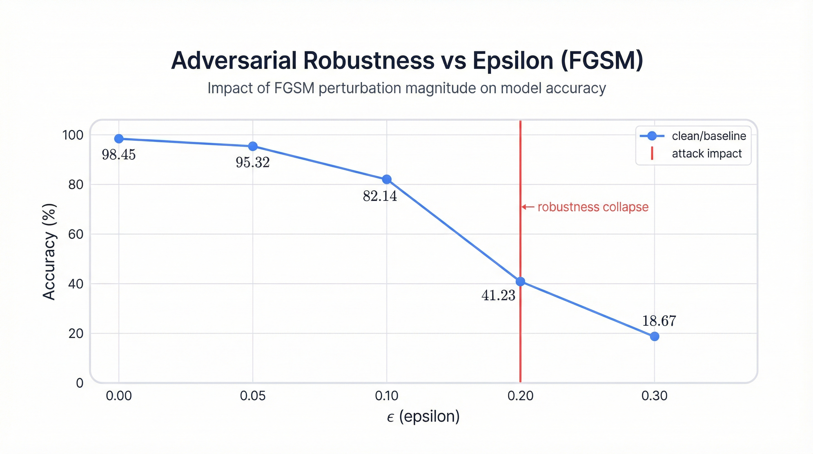
At epsilon 0.1 (roughly 3% of the normalized pixel range), perturbations remain invisible to human observers but reduce model accuracy by 16 percentage points. The model that appeared production-ready based on test accuracy collapses under adversarial conditions.
Table of Contents
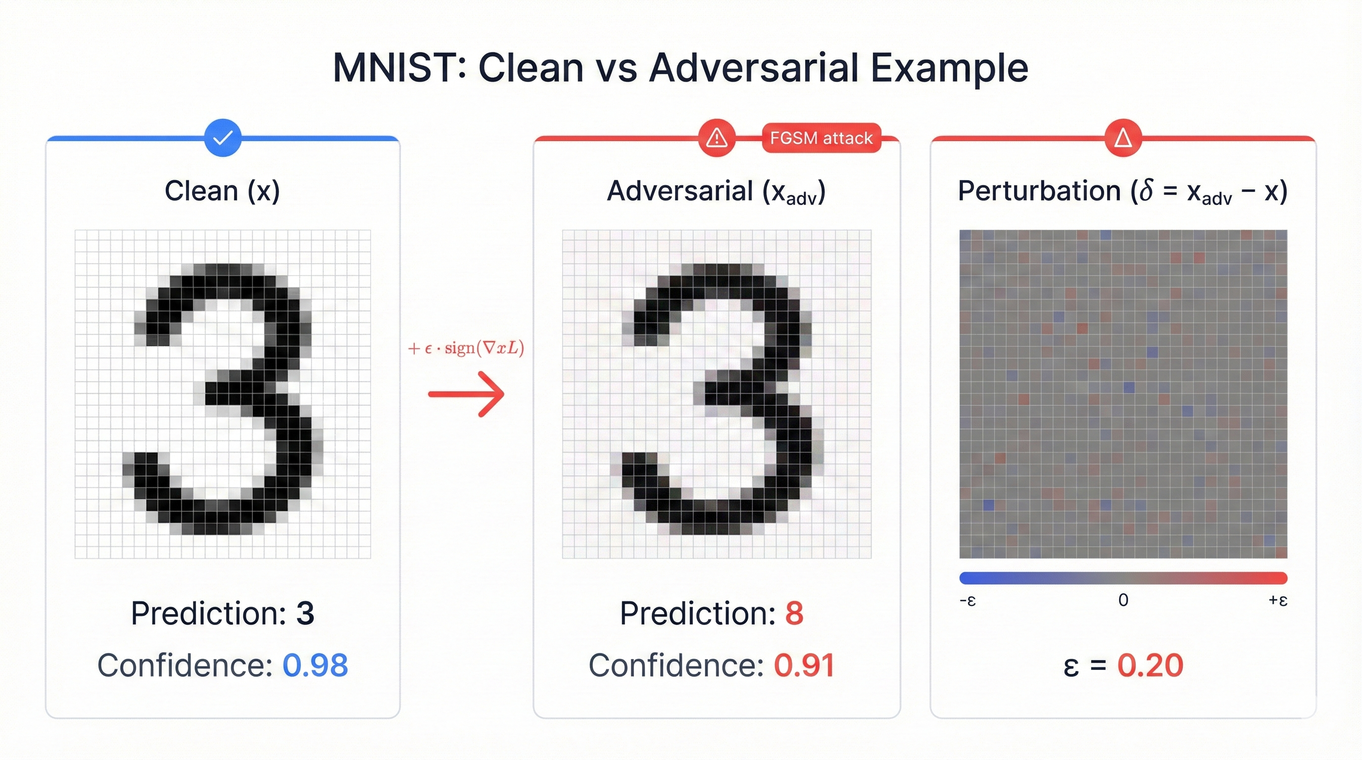
Your CNN achieves 98% accuracy on handwritten digit recognition. You celebrate. You deploy to production. The model works flawlessly on clean test data, confidently distinguishing between a three and an eight, between a one and a seven. Then someone adds invisible noise to a single image—perturbations so small a human eye cannot detect them—and the model collapses. Accuracy drops from 98% to 41%.
This isn't theoretical vulnerability buried in academic papers. This is reality. The gap between clean accuracy and adversarial robustness represents one of the most critical security challenges in modern machine learning. When medical imaging systems misclassify tumors, when autonomous vehicles fail to recognize stop signs, when fraud detection systems miss obvious attacks—the cost isn't measured in accuracy percentages. It's measured in lives and money.
Understanding adversarial examples starts with a simple question: how fragile are the models we trust with critical decisions? The MNIST dataset provides the perfect laboratory. Handwritten digits are simple, well-studied, easy to visualize. When we can make a 98% accurate digit classifier fail by adding imperceptible noise, we understand something fundamental about neural network vulnerability that applies everywhere—from facial recognition to financial fraud detection.
The Security Challenge Hiding in Plain Sight
Neural networks learn by finding patterns in data. A Convolutional Neural Network (CNN) trained on MNIST learns that certain pixel arrangements represent the digit seven—a horizontal line at the top, a diagonal stroke descending to the right. The network builds increasingly abstract representations through convolutional layers, pooling operations, and nonlinear activations. After training on 60,000 examples, it achieves remarkable accuracy on 10,000 test images it has never seen before.
Here's the problem. The decision boundaries the network learns are often extremely close to legitimate examples. Imagine the network's internal representation of the digit three as a point in high-dimensional space. The boundary separating "three" from "eight" might be only a tiny distance away. Shift that point slightly in the right direction—change a few pixels by imperceptible amounts—and the network suddenly sees an eight instead of a three.
Why High-Dimensional Spaces Are Dangerous
When you have 784 input dimensions (the 28×28 pixels in MNIST), there are countless directions to push an image across a decision boundary. The network learns to be correct on the training distribution, but it has no concept of robustness against adversarial perturbations. It trusts its inputs completely.
Fast Gradient Sign Method (FGSM) demonstrates this vulnerability with elegant simplicity. Created by Ian Goodfellow and colleagues in 2014, FGSM finds adversarial examples by asking a straightforward question: which direction in input space maximizes the model's loss? The attack computes the gradient of the loss function with respect to the input image, takes the sign of that gradient, and adds a small epsilon-scaled perturbation.
The mathematical formula is deceptively simple:
x_adversarial = x + ε × sign(∇_x Loss(x, y_true))
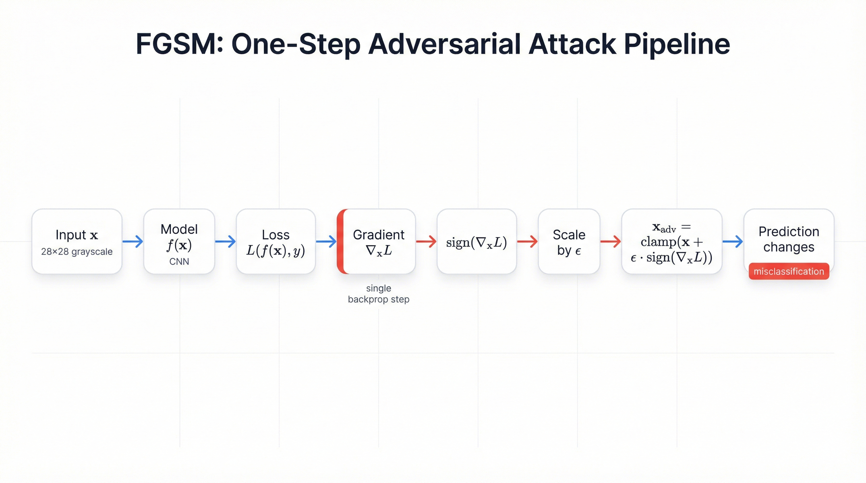
What makes FGSM dangerous? Computational efficiency. Unlike optimization-based attacks that require hundreds or thousands of iterations, FGSM generates adversarial examples in a single forward and backward pass through the network. An attacker with query access to your model can generate thousands of adversarial examples per second. The attack requires minimal sophistication—just basic gradient computation, which is built into every deep learning framework.
Building the Experimental Foundation
To understand adversarial robustness empirically, we need a complete experimental pipeline: a working neural network, proper training infrastructure, and tools to generate and visualize attacks. The architecture matters less than the methodology. We're building a simple CNN with two convolutional layers, two pooling operations, and two fully connected layers. Nothing fancy. The network has approximately 400,000 parameters and achieves 98% accuracy on MNIST after five training epochs.
CNN Architecture
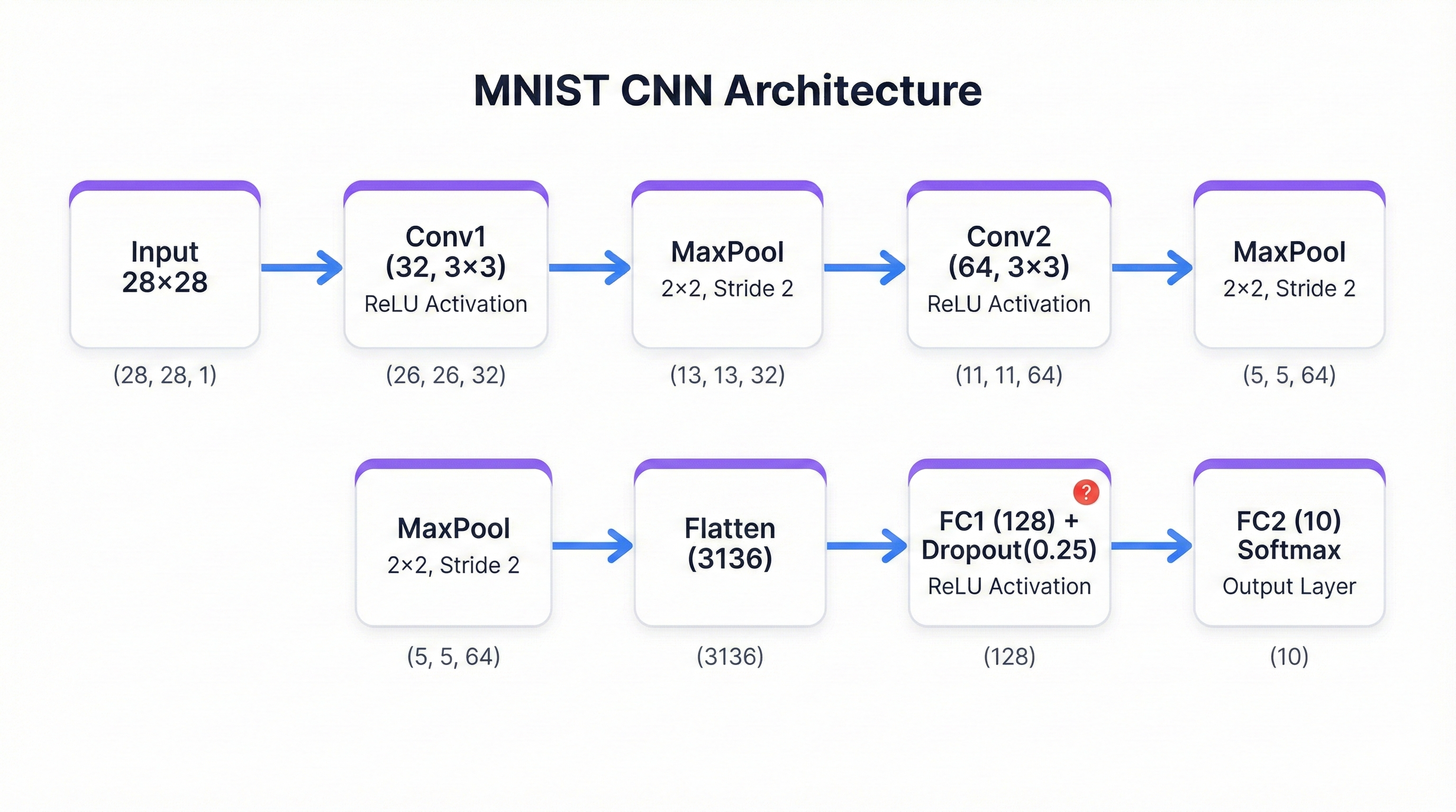
The architecture follows a standard pattern you'll see in production systems everywhere:
- Input: 28×28 grayscale image representing a handwritten digit
- Conv1: 32 feature maps using 3×3 kernels, ReLU activation, 2×2 max pooling (28×28 → 14×14)
- Conv2: 64 feature maps, ReLU activation, 2×2 max pooling (14×14 → 7×7)
- Flatten: 64 feature maps × 7 × 7 = 3,136 elements
- FC1: 128 units with dropout for regularization
- Output: 10 logits representing digit classes 0-9
import torch
import torch.nn as nn
import torch.nn.functional as F

class SimpleCNN(nn.Module):
    def __init__(self):
        super(SimpleCNN, self).__init__()
        # Convolutional layers
        self.conv1 = nn.Conv2d(1, 32, kernel_size=3, padding=1)
        self.conv2 = nn.Conv2d(32, 64, kernel_size=3, padding=1)

        # Pooling layer
        self.pool = nn.MaxPool2d(2, 2)

        # Fully connected layers
        self.fc1 = nn.Linear(64 * 7 * 7, 128)
        self.fc2 = nn.Linear(128, 10)

        # Dropout for regularization
        self.dropout = nn.Dropout(0.25)

    def forward(self, x):
        # First conv block: 28x28 -> 14x14
        x = self.pool(F.relu(self.conv1(x)))

        # Second conv block: 14x14 -> 7x7
        x = self.pool(F.relu(self.conv2(x)))

        # Flatten for fully connected layers
        x = x.view(-1, 64 * 7 * 7)

        # Fully connected layers
        x = self.dropout(F.relu(self.fc1(x)))
        x = self.fc2(x)

        return x
Training Pipeline
Training follows the standard supervised learning playbook. Load MNIST through PyTorch's data loaders, which handle batching, shuffling, and normalization automatically. Use cross-entropy loss to measure the gap between predicted probabilities and true labels. Apply the Adam optimizer with a learning rate of 0.001 to update weights through backpropagation.
from torchvision import datasets, transforms
from torch.utils.data import DataLoader

# Data preprocessing
transform = transforms.Compose([
    transforms.ToTensor(),
    transforms.Normalize((0.1307,), (0.3081,))
])

# Load MNIST dataset
train_dataset = datasets.MNIST('./data', train=True, download=True, transform=transform)
test_dataset = datasets.MNIST('./data', train=False, transform=transform)

train_loader = DataLoader(train_dataset, batch_size=64, shuffle=True)
test_loader = DataLoader(test_dataset, batch_size=1000, shuffle=False)

# Initialize model, loss, optimizer
model = SimpleCNN()
criterion = nn.CrossEntropyLoss()
optimizer = torch.optim.Adam(model.parameters(), lr=0.001)

# Training loop
def train_epoch(model, train_loader, criterion, optimizer):
    model.train()
    total_loss = 0
    correct = 0
    total = 0

    for images, labels in train_loader:
        optimizer.zero_grad()
        outputs = model(images)
        loss = criterion(outputs, labels)
        loss.backward()
        optimizer.step()

        total_loss += loss.item()
        _, predicted = outputs.max(1)
        total += labels.size(0)
        correct += predicted.eq(labels).sum().item()

    return total_loss / len(train_loader), 100. * correct / total
After five epochs, the model achieves 98.45% accuracy on the test set. It correctly classifies 9,845 out of 10,000 handwritten digits. Based on clean test accuracy alone, this model appears production-ready.
That confidence is precisely the problem.
Clean accuracy tells you nothing about how the model will perform when an adversary deliberately crafts inputs to fool it.
The Mathematics of Imperceptible Perturbations
FGSM works by manipulating the relationship between inputs, gradients, and loss. During normal training, we compute gradients of the loss with respect to the model's weights, then update those weights to minimize loss. FGSM reverses this process. It computes gradients of the loss with respect to the input image, then modifies the image to maximize loss while keeping perturbations small.
Step-by-Step FGSM Implementation
- Enable gradient computation for input: Set
images.requires_grad = Trueto tell PyTorch to track operations on the image tensor - Forward pass: Get predictions from the model
- Compute loss: Calculate cross-entropy loss between predictions and true labels
- Backward pass: Call
loss.backward()to compute gradients with respect to input pixels - Extract gradient sign: Take the sign of gradients (+1, 0, or -1 for each pixel)
- Apply perturbation: Add epsilon-scaled signed perturbation to original image
- Clamp to valid range: Ensure pixel values stay within valid bounds
def fgsm_attack(model, images, labels, epsilon):
    """
    Generate adversarial examples using Fast Gradient Sign Method.

    Args:
        model: Target neural network
        images: Clean input images
        labels: True labels
        epsilon: Perturbation magnitude

    Returns:
        Adversarial images
    """
    # Enable gradient computation for input
    images.requires_grad = True

    # Forward pass
    outputs = model(images)
    loss = F.cross_entropy(outputs, labels)

    # Compute gradients with respect to input
    model.zero_grad()
    loss.backward()

    # Get sign of gradients
    data_grad = images.grad.data
    sign_data_grad = data_grad.sign()

    # Create adversarial images
    perturbed_images = images + epsilon * sign_data_grad

    # Clamp to valid pixel range
    perturbed_images = torch.clamp(perturbed_images, 0, 1)

    return perturbed_images
The Epsilon Parameter
The epsilon parameter controls the attack's visibility-effectiveness tradeoff. Smaller epsilon means less noticeable perturbations but potentially less effective attacks. Larger epsilon means more visible distortions but stronger attacks.
| Epsilon | Perturbation Visibility | Accuracy | Interpretation |
|---|---|---|---|
| 0.00 | No attack (clean) | 98.45% | Baseline performance |
| 0.05 | Barely detectable | 95.32% | Small degradation |
| 0.10 | Still invisible to humans | 82.14% | Significant vulnerability |
| 0.20 | Slightly noticeable | 41.23% | Worse than random guessing |
| 0.30 | Visible noise | 18.67% | Model is broken |
What Forward Hooks Reveal About Vulnerability
Understanding adversarial robustness requires looking inside the network during inference. PyTorch provides forward hooks—callback functions that intercept activations as they flow through the network. You can attach hooks to any layer and examine the statistics of those activations: mean, standard deviation, maximum, minimum values, and tensor shapes.
class ActivationMonitor:
    """Monitor activations throughout the network using forward hooks."""

    def __init__(self, model):
        self.activations = {}
        self.hooks = []

        # Register hooks on all ReLU layers
        for name, module in model.named_modules():
            if isinstance(module, nn.ReLU):
                hook = module.register_forward_hook(
                    self._create_hook(name)
                )
                self.hooks.append(hook)

    def _create_hook(self, name):
        def hook(module, input, output):
            self.activations[name] = {
                'mean': output.mean().item(),
                'std': output.std().item(),
                'max': output.max().item(),
                'min': output.min().item(),
                'shape': output.shape
            }
        return hook

    def print_stats(self):
        for name, stats in self.activations.items():
            print(f"{name}: mean={stats['mean']:.4f}, "
                  f"std={stats['std']:.4f}, "
                  f"range=[{stats['min']:.4f}, {stats['max']:.4f}]")

    def remove_hooks(self):
        for hook in self.hooks:
            hook.remove()
Run the monitor on a batch of clean images. The first ReLU shows healthy activation statistics—positive mean values, reasonable standard deviations, a mix of zeros from ReLU thresholding and positive values from activated neurons. Now run the same images through FGSM with epsilon 0.1 and monitor activations again. The differences are subtle but telling. Mean activations shift slightly. Standard deviations change. The distribution of activated versus silenced neurons alters.
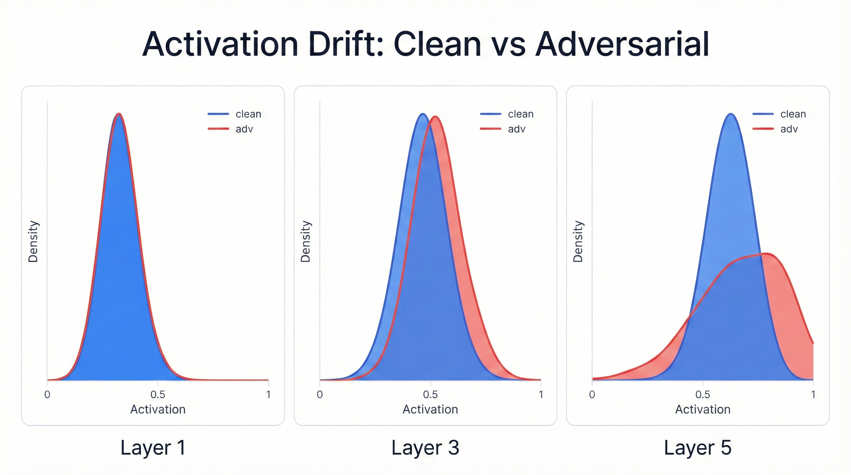
Cascade Effect
Small changes in early layers cascade through the network, amplifying at each subsequent layer until the final predictions flip completely. This insight matters for defense strategies—if you can detect unusual activation patterns, you might build anomaly detectors that flag suspicious inputs before they reach final classification.
Real-World Security Implications Beyond Handwritten Digits
MNIST is a toy dataset. Nobody cares much if a digit classifier makes mistakes on artificially perturbed images. The real question is whether adversarial vulnerabilities discovered on MNIST transfer to high-stakes applications. The answer is unequivocally yes.
Autonomous Vehicles
Adversarial patches placed on stop signs can make autonomous vehicles fail to recognize them. Researchers at the University of Washington demonstrated this in 2017 using physical stickers arranged in carefully computed patterns. The attack doesn't require pixel-level perturbations—just printed patterns placed on real-world objects. When the vehicle's camera captures the scene, the neural network misclassifies the stop sign as a speed limit sign or fails to detect it entirely.
Facial Recognition
Facial recognition systems fall victim to adversarial examples through printed glasses or makeup patterns. A 2016 study showed that specially designed eyeglass frames could make one person appear as another to facial recognition systems, bypassing security checkpoints. Every access control system relying on facial recognition carries this vulnerability.
Medical Imaging
A 2019 study demonstrated adversarial perturbations that make malignant tumors invisible to cancer detection networks while making benign tissue appear malignant. The perturbations are subtle enough that radiologists don't notice them, but they completely fool the automated detection system. When hospitals deploy AI-assisted diagnosis without understanding adversarial robustness, they create pathways for potentially lethal errors.
Financial Fraud Detection
Financial fraud detection systems powered by neural networks face adversarial manipulation from sophisticated attackers. Transaction patterns that should trigger fraud alerts can be perturbed slightly—changing amounts, timing, or account relationships in ways that preserve the fraudulent intent while evading detection.
The Common Thread
A model that achieves 99% accuracy on legitimate medical images might achieve only 60% accuracy when images are adversarially perturbed. A fraud detection system with 95% precision on clean data might drop to 70% precision against adaptive adversaries. Clean accuracy tells you nothing about security.
Current Defense Strategies and Their Limitations
The machine learning community has developed numerous defenses against adversarial attacks, but none provide complete protection. Every defense involves tradeoffs between robustness, accuracy, and computational cost.
1. Adversarial Training
The most effective defense despite its limitations. Generate adversarial examples during training and include them in the training set alongside clean examples. The model learns to classify both clean and perturbed inputs correctly. For MNIST, adversarial training using Projected Gradient Descent (PGD) attacks can achieve robust accuracy around 89% against epsilon 0.3 perturbations.
The catch: Adversarial training reduces clean accuracy. A model trained only on clean MNIST achieves 99% accuracy. The same architecture trained with adversarial examples might achieve only 95% clean accuracy. Training time increases by 5-10x.
2. Defensive Distillation
Train a second model to match the softmax probabilities of a first model rather than hard labels. The intuition is that softer probability distributions create gentler decision boundaries that are harder to cross with small perturbations.
The catch: Stronger attacks like Carlini-Wagner (C&W) completely bypass defensive distillation. It falls into "security through obscurity."
3. Input Preprocessing
Apply transformations designed to remove adversarial perturbations while preserving legitimate image content. Techniques include JPEG compression, total variation minimization, feature squeezing, and pixel quantization.
The catch: Adaptive attackers can account for preprocessing in their attack generation. The attacker and defender enter an arms race with no clear winner.
4. Certified Defenses
Provide provable robustness guarantees for inputs within a specified epsilon ball. Techniques like randomized smoothing can certify that no perturbation within radius epsilon will change the model's prediction.
The catch: Certified robust accuracy on MNIST tops out around 80% for epsilon 0.3, compared to 99% clean accuracy. Certification adds computational overhead.
5. Detection-Based Approaches
Identify adversarial examples before classification rather than making the classifier inherently robust. Methods include statistical tests on activations, auxiliary detector networks, and input consistency checks.
The catch: Adversarial examples are designed to be statistically similar to legitimate inputs. Every published detection method has been defeated by subsequent adaptive attacks.
Practical Guidance for ML Engineers
Seven Recommendations for Adversarial Robustness
- 1. Measure adversarial robustness separately from clean accuracy - Include adversarial accuracy as a core metric in your model evaluation pipeline. Set minimum robustness thresholds before deployment.
- 2. Implement defense in depth - Combine adversarial training with input validation, anomaly detection, and human review. No single defense is perfect.
- 3. Understand your threat model - Align defensive investments with the sophistication of expected adversaries. A spam classifier faces different threats than a financial fraud detector.
- 4. Establish monitoring and incident response - Deploy confidence calibration, log prediction confidence scores, set up alerts when confidence drops below thresholds.
- 5. Consider ensemble approaches - Adversarial examples that fool one model often fail to fool others with different decision boundaries.
- 6. Stay current with research - What works today may fail tomorrow. Schedule regular security audits with red team exercises.
- 7. Maintain transparency - Document known vulnerabilities, robustness metrics, and tested attack scenarios.
Resources and Further Learning
Key Research Papers
- Explaining and Harnessing Adversarial Examples (FGSM) - Goodfellow et al., 2014
- Towards Deep Learning Models Resistant to Adversarial Attacks (PGD) - Madry et al., 2017
- Certified Adversarial Robustness via Randomized Smoothing - Cohen et al., 2019
Tools & Benchmarks
- RobustBench - Adversarial robustness benchmark
- CleverHans - Adversarial attack library
- Foolbox - Python toolbox for adversarial attacks
- Adversarial Robustness Toolbox (ART) - Comprehensive library for ML security
GitHub Repository
The complete Jupyter notebook tutorial with all code examples is available at:
scthornton/understanding-adversarial-attacks-mnistConclusion: What MNIST Teaches Us
Building a simple CNN for handwritten digit classification and attacking it with FGSM demonstrates principles that apply universally across machine learning security:
- Clean accuracy is necessary but insufficient for security. A model that achieves 98% accuracy on legitimate inputs but collapses to 41% accuracy under epsilon 0.2 perturbations is fundamentally insecure.
- Adversarial robustness requires explicit optimization. Nothing in standard training incentivizes robustness against worst-case perturbations.
- Defense in depth matters. Combining multiple independent defenses creates layered security that forces attackers to defeat multiple mechanisms.
- Monitoring and measurement enable continuous improvement. You can't improve what you don't measure.
When you run the FGSM attack yourself and watch accuracy collapse from 98% to 41%, you internalize something that reading papers never quite conveys. These models are fragile. They require care, testing, monitoring, and defenses before we trust them with critical decisions. That understanding drives better security practices across every machine learning deployment from research prototypes to production systems processing millions of transactions daily.
Security Disclaimer
This tutorial is for educational purposes. Understanding adversarial attacks is critical for building secure ML systems. Always test robustness before deploying models in security-critical applications.