The Beautiful Geometry Behind SVMs
Support Vector Machines have an elegant core idea. Don't just find any decision boundary that separates your data. Find the best one. The "best" boundary maximizes the margin between classes, creating the most robust classifier possible.
Key Concept: Understanding this foundational concept is essential for mastering the techniques discussed in this article.
The Optimal Hyperplane: Drawing the Perfect Line
SVMs find the best possible decision boundary to separate different classes. This boundary is called a hyperplane—a line in 2D, a plane in 3D, or its higher-dimensional equivalent.
Imagine a scatter plot. Red dots. Blue dots. Clearly separable. You could draw many different lines to divide red from blue. Which line is best?
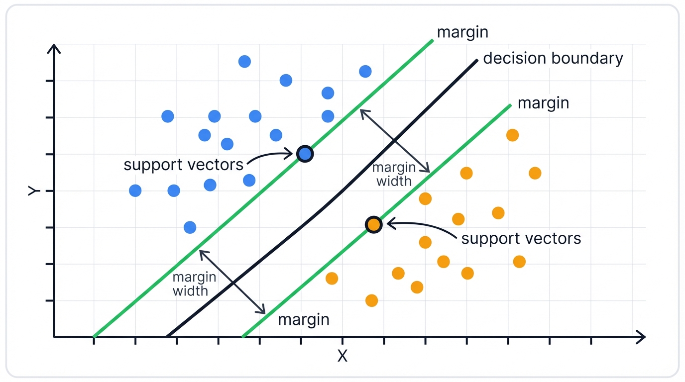
SVM's answer is brilliant. Choose the line farthest from both classes. This creates the widest possible "street" between the colors.
The margin is the width of this street. The distance between the decision boundary and the nearest data points from either class. SVM finds the hyperplane that maximizes this margin.
Why does this matter? Simple. A classifier with a larger margin generalizes better to new data. More confident. More robust. Think of it as giving yourself maximum safety buffer when making decisions.
Picture this scenario. Red and blue dots on a page. You could draw many lines—some hugging the red cluster, others barely missing the blue points.
SVM ignores all mediocre options. It finds one line. The one line that's maximally distant from both the closest red dot and closest blue dot. This line runs down the middle of the widest possible street between the clusters.
That street is the margin. Maximizing it makes SVMs special.
Support Vectors: The Points That Matter Most
Support vectors are data points lying exactly on the margin boundaries. The "edges of the street." These are the most difficult points to classify. The most important for the algorithm.
Here's what's remarkable. Only these support vectors determine the decision boundary. You could delete every other training point. The optimal hyperplane wouldn't change. The entire model is literally "supported" by just these few critical points.
This is why it's called Support Vector Machine. The support vectors are the heroes of the story.
Hard Margin vs. Soft Margin SVMs
Hard Margin SVM represents the original, mathematically pure version. It assumes perfect linear separability. This strict approach draws a hyperplane with zero tolerance for mistakes. No training points can fall within the margin or on the wrong side. Elegant in theory. Problematic in practice. Why? Real-world data is messy. Noise. Outliers. Overlapping class distributions. Perfect separation? Impossible.
Soft Margin SVM provides the practical solution. It introduces flexibility. Allows some classification mistakes. Trades off margin width against errors. Uses a penalty parameter to control misclassification tolerance while seeking optimal balance. This flexibility makes SVMs robust to noisy, real-world data while maintaining their theoretical foundation.
Real data is messy. Noise. Outliers. Overlapping classes. Rigid boundary enforcement becomes counterproductive. The Soft Margin SVM addresses this reality through a more flexible formulation that permits controlled misclassification by introducing slack variables (denoted by ξ) that measure how much each data point violates ideal margin requirements. The algorithm's objective function incorporates a penalty term for these violations, creating a fundamental trade-off. Maximize the geometric margin? Or minimize training errors? This trade-off is controlled by the regularization hyperparameter C, which determines how heavily margin violations are penalized. By allowing this "soft" margin, SVMs become robust to outliers and applicable to most practical problems where perfect class separation is neither possible nor desirable.
Classification and Learning Paradigm positions Support Vector Machines as a supervised learning method. The algorithm learns from training datasets where each data point comes with a correct class label. Its fundamental task? Learn a general decision rule from labeled training data that can accurately assign class labels to new, previously unseen data points. While the core SVM framework has been adapted for other tasks—regression through Support Vector Regression (SVR), unsupervised learning through Support Vector Clustering—its primary application and greatest success remains in classification problems where clear class boundaries can be identified and optimized.
Historical Foundations: From the Generalized Portrait to Modern SVM
Popular narratives place SVM invention in the 1990s at AT&T Bell Labs. Wrong. The algorithm's roots extend much deeper. Into Soviet mathematical research during the Cold War era. Vladimir Vapnik and Alexey Chervonenkis developed the fundamental concepts at Moscow's Institute of Control Sciences. Beginning in 1962. First publishing results in 1964. Their original framework? The "Generalized Portrait." Essentially the linear hard-margin SVM, conceived as an algorithm to find an optimal "portrait" vector that could distinguish one class from another through geometric optimization principles.
This early work represented far more than algorithmic invention. It established the foundation for a new statistical learning theory. Vapnik and Chervonenkis co-developed what became Vapnik-Chervonenkis (VC) theory and the principle of Structural Risk Minimization (SRM), fundamentally changing how machine learning approaches generalization. While contemporary algorithms focused on Empirical Risk Minimization (ERM) that simply minimized training error, Vapnik and Chervonenkis recognized this approach's tendency toward overfitting. SRM instead seeks to minimize an upper bound on generalization error by balancing training accuracy against model complexity as quantified by the VC dimension. The SVM's core objective of maximizing the geometric margin? A direct and elegant implementation of SRM principles. It provides mathematically rigorous guarantees against overfitting that distinguished it from heuristic approaches of its era.
The algorithm gained widespread international recognition after Vapnik moved to AT&T Bell Labs in the United States in the early 1990s. This move coincided with intense research in machine learning, particularly in character recognition. The pivotal breakthrough that catapulted SVMs to prominence? The 1992 paper by Bernhard Boser, Isabelle Guyon, and Vladimir Vapnik. They introduced the kernel trick. This innovation allowed the linear algorithm to create non-linear classifiers by implicitly mapping data into higher-dimensional space. This transformed the SVM from a niche linear method into an exceptionally versatile and powerful tool capable of handling complex, non-linear datasets. The modern, standard soft-margin formulation, which added robustness to noise and non-separability, was later proposed by Corinna Cortes and Vapnik in a highly influential 1995 paper.
The enduring appeal and initial success of SVMs can be attributed to their simple and powerful geometric intuition. Unlike statistical models such as logistic regression, which are founded on probabilistic principles, the SVM is fundamentally about finding optimal geometric separation. This geometric foundation leads directly to the concepts of support vectors and margin maximization. The objective of the algorithm? Maximize a physical distance—the margin, equivalent to $2 / |\mathbf{w}|$. This goal is distinct from maximizing a likelihood function. This framework's strength lies in problems where a clear, albeit potentially complex, geometric boundary exists. This also explains its initial development as a "pattern recognition" tool, a task that is inherently visual and geometric.
However, while geometric ideas are intuitive, the true differentiator that established SVMs as a cornerstone of modern machine learning is their rigorous foundation in Statistical Learning Theory and Structural Risk Minimization. This provided mathematical justification for why maximizing the margin leads to better generalization on unseen data. A critical problem that plagued other contemporary methods like neural networks, which were seen as heuristic, prone to overfitting, and susceptible to local minima. The SRM principle explicitly balances training error against model complexity. The SVM's objective function is a direct implementation of this idea. This strong theoretical backing, combined with the convex nature of its optimization problem which guarantees a unique, global optimal solution, gave researchers immense confidence in the method's robustness and its ability to avoid overfitting, representing a significant advantage over other approaches of the time.
The Mathematical Architecture of SVMs
This section deconstructs the mathematical engine of Support Vector Machines. Translating geometric intuition into a formal optimization problem. It covers the primal and dual formulations, essential for understanding both the training process and the mechanics of the kernel trick—the innovation that allows SVMs to handle non-linear data.
The Primal Optimization Problem: Maximizing the Margin
The core task of a linear SVM? Find the optimal separating hyperplane. In a d-dimensional feature space, any hyperplane can be defined by the equation:
$$\mathbf{w}^T\mathbf{x} + b = 0$$
where $\mathbf{w}$ is a d-dimensional weight vector normal (perpendicular) to the hyperplane, $\mathbf{x}$ is a data point, and $b$ is a scalar bias term that determines the hyperplane's offset from the origin.
For binary classification, class labels $y$ are conventionally set to $-1$ and $+1$. A new data point $\mathbf{x}$ is classified based on which side of the hyperplane it falls. Determined by the sign of the decision function $f(\mathbf{x}) = \mathbf{w}^T\mathbf{x} + b$.
The margin is defined by two parallel hyperplanes: $\mathbf{w}^T\mathbf{x} + b = 1$ and $\mathbf{w}^T\mathbf{x} + b = -1$. The distance between these two planes? It can be shown to be $2 / |\mathbf{w}|$. To achieve maximum possible margin, the algorithm must minimize the norm of the weight vector, $|\mathbf{w}|$. For mathematical convenience—particularly to make the optimization problem quadratic and convex—this is equivalent to minimizing $\frac{1}{2}|\mathbf{w}|^2$.
This minimization is performed subject to a constraint. All training data points must be correctly classified and lie outside the margin. This constraint is expressed as:
$$y_i(\mathbf{w}^T\mathbf{x}_i + b) \geq 1 \text{ for all training samples } i = 1, \ldots, n$$
This formulation is the primal problem for a hard-margin SVM.
The Soft Margin Formulation: Introducing Slack and the Hinge Loss
The hard-margin formulation is brittle. It assumes perfect linear separability. To make the algorithm practical for real-world data—which is noisy and overlapping—the soft-margin formulation introduces non-negative slack variables, $\xi_i \geq 0$, for each data point $\mathbf{x}_i$. These variables relax the hard constraint. Allowing some points to violate the margin. The constraint is modified to:
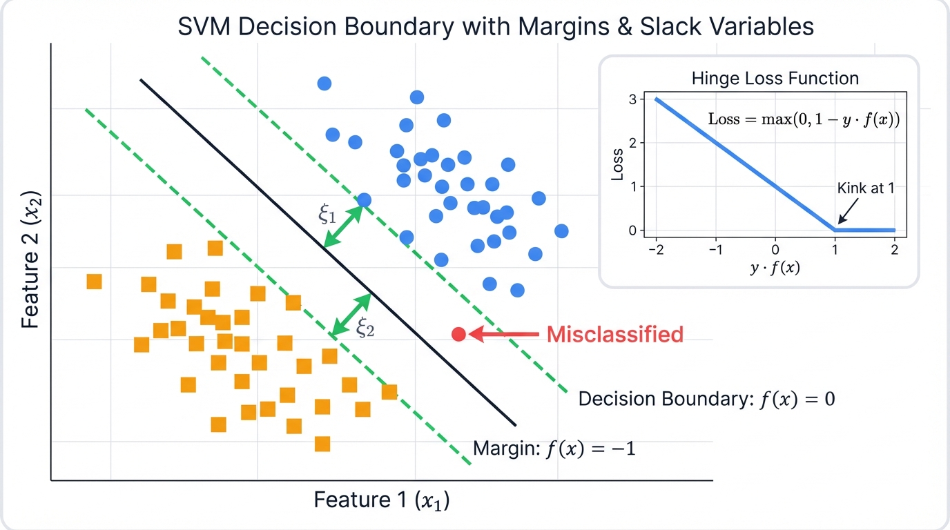
$$y_i(\mathbf{w}^T\mathbf{x}_i + b) \geq 1 - \xi_i$$
If $\xi_i = 0$, the point is correctly classified. On or outside the margin. If $0 < \xi_i \leq 1$, the point is within the margin but still on the correct side of the hyperplane. If $\xi_i > 1$, the point is misclassified.
To control these violations, the objective function is updated to include a penalty term. The new objective? Minimize:
$$\frac{1}{2}\|\mathbf{w}\|^2 + C \sum_{i=1}^{n} \xi_i$$
The hyperparameter $C > 0$ is the regularization parameter that controls the trade-off. Maximize the margin? Or minimize classification error? A high value of $C$ imposes a large penalty for margin violations. Forces the model to classify as many points correctly as possible. This can lead to a narrower margin and potential overfitting. Conversely, a small value of $C$ allows for more margin violations. In favor of a wider, simpler margin. This can improve generalization but may underfit the training data.
This entire formulation is an elegant implementation of minimizing a specific loss function. The hinge loss. Defined as $L(y, f(\mathbf{x})) = \max(0, 1 - y \cdot f(\mathbf{x}))$, plus a regularization term $\lambda|\mathbf{w}|^2$ (where $\lambda$ is related to 1/C). The hinge loss is zero for points correctly classified outside the margin. For any point that violates the margin? The loss increases linearly with its distance from the correct margin boundary.
The Lagrangian Dual Formulation: A Path to the Kernel
The primal problem, while convex, is a constrained optimization problem. Difficult to solve directly. Especially when the kernel trick is introduced. A more powerful and elegant solution? Reformulate using the method of Lagrange multipliers. This leads to the dual problem.
By introducing non-negative Lagrange multipliers $\alpha_i \geq 0$ for each constraint, we can solve for $\mathbf{w}$ and $b$ and substitute them back into the Lagrangian. This process transforms the original minimization problem into a maximization problem with respect to the $\alpha_i$ variables. The dual objective function to be maximized:
$$L_D(\boldsymbol{\alpha}) = \sum_{i=1}^{n} \alpha_i - \frac{1}{2} \sum_{i=1}^{n} \sum_{j=1}^{n} \alpha_i \alpha_j y_i y_j (\mathbf{x}_i^T \mathbf{x}_j)$$
subject to the constraints:
$$\sum_{i=1}^{n} \alpha_i y_i = 0 \quad \text{and} \quad 0 \leq \alpha_i \leq C$$
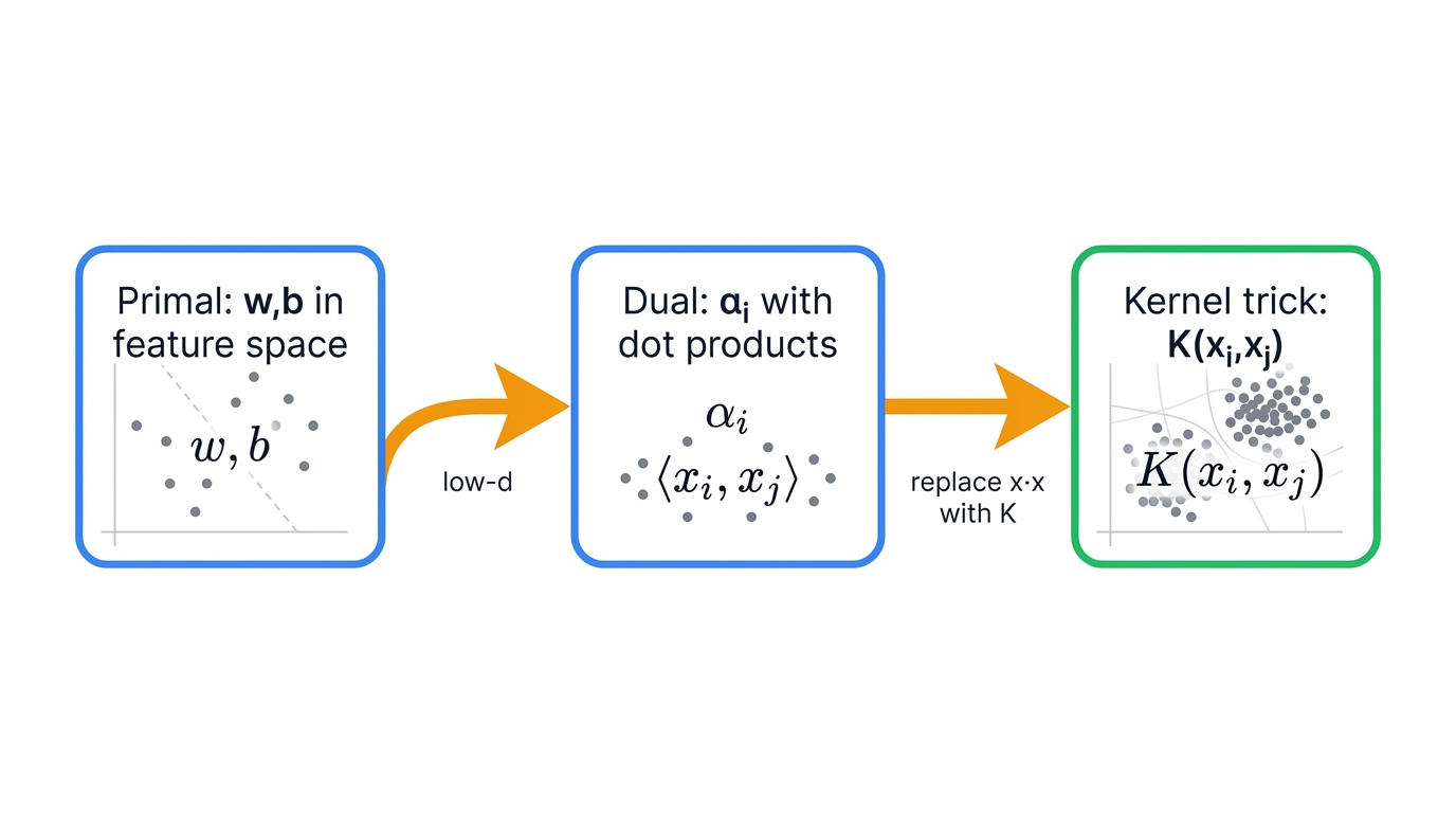
This dual formulation has a profound and critical property. The training data points $\mathbf{x}_i$ only ever appear in the form of dot products: $\mathbf{x}_i^T \mathbf{x}_j$. This specific structure is the key. It unlocks the kernel trick, allowing SVMs to operate in high-dimensional spaces efficiently.
The transformation from primal to dual is not merely mathematical convenience. It is the single most important theoretical step that unleashes the full power of SVMs. The primal problem is defined in terms of $\mathbf{w}$ and $b$ in the feature space. The dimensionality of $\mathbf{w}$ equals the number of features. If one were to map data to a very high-dimensional or even infinite-dimensional space, computing and storing $\mathbf{w}$ would become intractable. The dual problem, however, is formulated in terms of the multipliers $\alpha_i$. The number of variables equals the number of samples, not features. Crucially, the feature vectors $\mathbf{x}$ only appear inside dot products within the dual objective function. This means the algorithm never needs to know the explicit coordinates of the data in the high-dimensional space. It only needs a way to compute their dot products. This is the exact prerequisite for the kernel trick. Making the dual formulation the essential enabling mechanism for powerful non-linear classification.
Karush-Kuhn-Tucker (KKT) Conditions
The Karush-Kuhn-Tucker (KKT) conditions are a set of necessary and sufficient conditions for optimality in a constrained optimization problem like the SVM. For the SVM, one of the most important KKT conditions is the dual complementarity condition. It states that for each training point $i$:
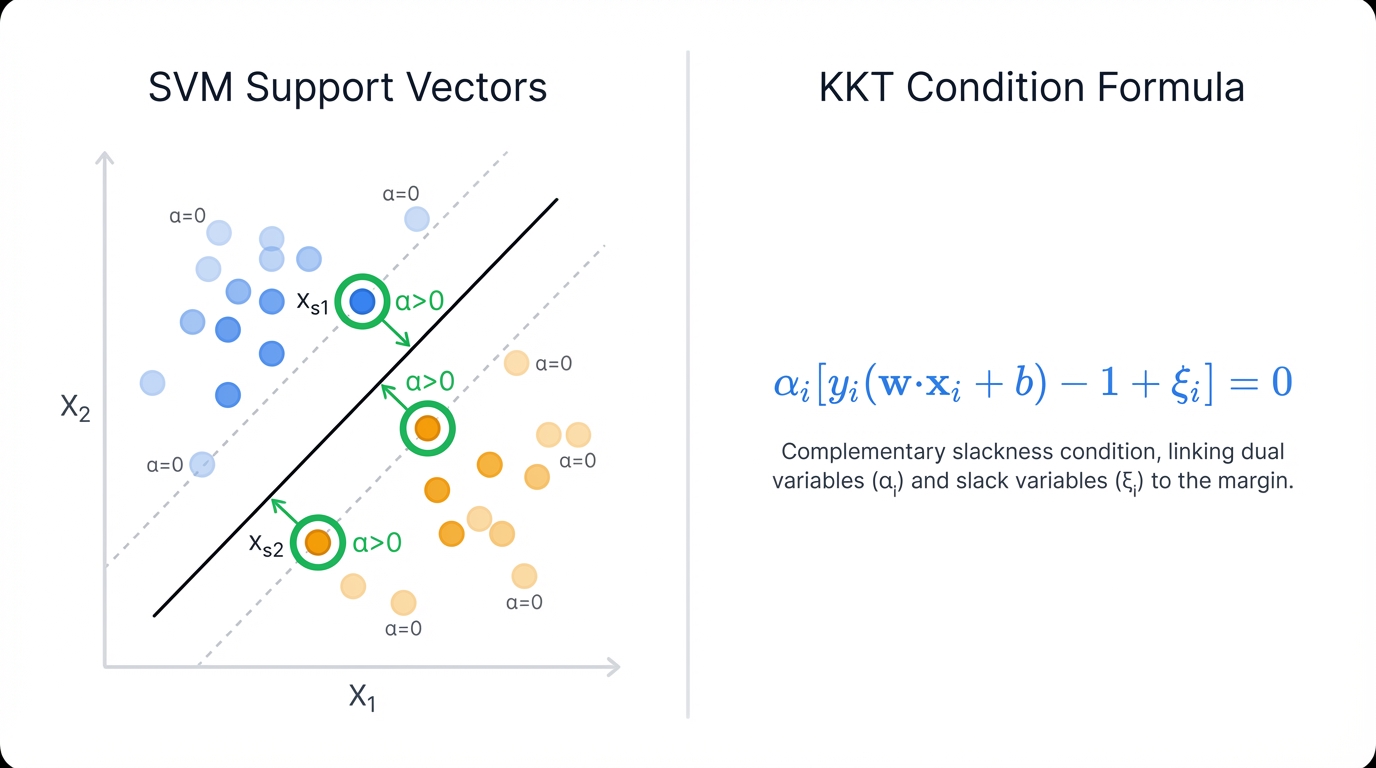
$$\alpha_i \left[y_i(\mathbf{w}^T\mathbf{x}_i + b) - 1 + \xi_i\right] = 0$$
This condition reveals a fundamental property of the solution. For the multiplier $\alpha_i$ to be non-zero ($\alpha_i > 0$), the term in the brackets must be zero. This means $y_i(\mathbf{w}^T\mathbf{x}_i + b) = 1 - \xi_i$. These are precisely the points that lie on the margin (if $\xi_i = 0$) or violate the margin (if $\xi_i > 0$). All other points? Correctly classified. Lying strictly outside the margin. Will have $\alpha_i = 0$.
Therefore, the data points with non-zero Lagrange multipliers are the support vectors. This provides mathematical proof for the geometric intuition that the optimal hyperplane is determined solely by this small subset of the training data. The final weight vector can be expressed as a linear combination of only the support vectors: $\mathbf{w} = \sum_{i \in SV} \alpha_i y_i \mathbf{x}_i$.
The hyperparameter $C$ serves as the explicit lever for controlling the model's complexity. Consequently, the fundamental bias-variance trade-off. The objective function, $\min \left( \frac{1}{2}|\mathbf{w}|^2 + C \sum \xi_i \right)$, directly balances two competing goals. The first term, $\frac{1}{2}|\mathbf{w}|^2$, is inversely related to the margin width. Minimizing it leads to a wider margin. A simpler, less complex decision boundary (higher bias, lower variance). The second term, $C \sum \xi_i$, represents the cost of misclassification. Minimizing it leads to lower training error (lower bias, higher variance). The parameter $C$ directly mediates this conflict. A very large $C$? Forces the model to minimize training error at all costs. Potentially creating a narrow-margin, complex boundary that overfits the data (low bias, high variance). Conversely, a very small $C$ prioritizes a large margin. Even at the expense of misclassifying many training points. Resulting in a simpler model that may underfit but generalize better (high bias, low variance). Understanding $C$ as the knob that tunes this trade-off? Essential for effective practical implementation of SVMs.
Practical Implementation
This section transitions from mathematical theory to practical considerations. Detailing the requirements for data preparation, computational costs involved, and the ecosystem of software tools available for deploying SVM models.
Data Requirements
Data Types that SVMs can process span a wide range of formats. Provided they are converted into appropriate numerical representations. Numerical data works natively. The algorithm is designed to operate on continuous feature vectors. Categorical data requires encoding. One-hot encoding converts each category into binary features. Dummy variable encoding creates numerical representations while avoiding assumptions about ordinal relationships. Text data represents one of SVMs' greatest strengths. Particularly for classification tasks. Raw text is converted into high-dimensional numerical vector spaces using methods like Bag-of-Words, TF-IDF (Term Frequency-Inverse Document Frequency), or modern word embeddings. The resulting sparse vectors? Handled efficiently by SVM algorithms. Image data can be processed by extracting features using domain-specific algorithms like HOG (Histogram of Oriented Gradients) or SIFT (Scale-Invariant Feature Transform) that capture important visual patterns. Or by flattening raw pixel values into high-dimensional vectors that SVMs can process directly.
Data Preprocessing represents a critical requirement. Not merely a best practice. Feature scaling stands as the most important preprocessing step. Why? SVMs rely fundamentally on calculating distances between data points to define optimal margins. Making them extremely sensitive to feature scale differences. When features have vastly different numerical ranges, those with larger scales will dominate distance calculations. Inappropriately influencing final hyperplane positioning. Essentially breaking the algorithm's geometric foundation. Essential scaling approaches include standardization (converting to zero mean and unit variance) or normalization (scaling to specific ranges like [0,1]). Failure to properly scale data? Potentially invalidates the entire geometric premise underlying SVM operation. Missing value handling requires explicit preprocessing. SVMs cannot natively process incomplete data. Typically addressed through imputation methods like mean, median, or sophisticated model-based predictions. Or through sample removal when missing values are rare and their elimination doesn't significantly impact dataset representativeness.
Ideal Dataset Sizes fundamentally determine SVM feasibility and performance characteristics across different application scenarios. Small to medium datasets (1,000 to 100,000 samples) represent SVMs' optimal operating range. They consistently demonstrate exceptional performance. Often outperforming more complex algorithms due to their robust theoretical foundation and resistance to overfitting. High-dimensional data scenarios where feature count exceeds sample count (p > n) showcase SVMs' particular strength. Making them exceptionally effective for fields like bioinformatics and text analysis where this condition occurs. Large datasets (over 100,000 samples) present increasing computational challenges for standard kernelized SVMs. Training times become prohibitively long due to the algorithm's quadratic to cubic complexity scaling with sample size. Very large datasets (over one million samples) typically require alternative algorithms such as logistic regression with stochastic gradient descent, tree-based ensembles like LightGBM, or deep neural networks that offer superior scalability characteristics for big data applications.
Computational Complexity
Computational Complexity represents a defining characteristic. It fundamentally determines SVM applicability across different data scales and problem types. Training complexity for kernelized SVMs involves solving computationally intensive quadratic programming problems. Standard Sequential Minimal Optimization (SMO) algorithms exhibit time complexity between O(n²d) and O(n³d). Where n represents training samples and d represents features. This quadratic or cubic dependence on sample count creates the primary scalability barrier. Preventing SVMs from handling very large datasets effectively. Linear SVMs benefit from much faster specialized solvers like those in LIBLINEAR. With complexity closer to O(nd). Making them viable for larger datasets when linear separation suffices.
Prediction complexity for trained SVM models depends directly on the number of support vectors (n_sv) identified during training. Kernel SVMs require O(n_sv × d) time for each prediction. They must compute kernel functions between new points and every support vector. Though sparse solutions with n_sv << n can achieve very fast prediction times. Linear SVMs achieve optimal O(d) prediction complexity through simple dot product computation with the learned weight vector. Making them extremely efficient for real-time applications.
Space complexity during training centers on kernel matrix storage requirements of size n × n. Leading to O(n²) space complexity that becomes prohibitive for large datasets. However, the final trained model requires only support vectors and their corresponding coefficients. Resulting in O(n_sv × d) space complexity. Can be very memory-efficient when the algorithm finds sparse solutions with relatively few support vectors.
The power of SVMs, derived from kernel methods and convex optimization, comes at a direct and steep computational cost. This perfectly illustrates the "no free lunch" theorem in machine learning. The $O(n^2)$ or $O(n^3)$ training complexity is not merely an implementation detail. It's a fundamental consequence of the algorithm's need to solve a quadratic program involving all pairs of data points to construct the kernel matrix. This quadratic relationship is the primary bottleneck. Consequently, while SVMs are theoretically elegant and highly effective on complex, high-dimensional, but moderately sized datasets, this very elegance prevents them from scaling to the "big data" regime. Where simpler, iterative algorithms like logistic regression (trained with SGD) or deep neural networks excel. This creates a clear decision boundary for practitioners: if the number of samples is very large, the theoretical guarantees of SVM may be outweighed by the practical impossibility of training the model in a reasonable timeframe.
Popular Libraries and Frameworks
Popular Libraries and Frameworks provide a rich ecosystem. Making SVMs accessible to practitioners across diverse platforms and programming languages through highly optimized implementations. LIBSVM and LIBLINEAR represent the foundational software packages developed by Chih-Jen Lin and colleagues at National Taiwan University. Providing highly optimized, open-source C++ libraries that form the backbone of most SVM implementations worldwide. LIBSVM implements the Sequential Minimal Optimization (SMO) algorithm for comprehensive kernelized SVM capabilities including C-SVC, nu-SVC, epsilon-SVR, and one-class SVM variants. Establishing itself as the de facto standard for non-linear SVM implementation. LIBLINEAR focuses specifically on large-scale linear classification with significantly faster performance than LIBSVM for linear problems. Also supporting logistic regression for broader applicability.
Scikit-learn for Python provides the most widely used machine learning interface. Offering user-friendly, consistent APIs for SVMs through modules that wrap the optimized LIBSVM and LIBLINEAR libraries while adding Python's accessibility and integration capabilities. The sklearn.svm.SVC module handles support vector classification using kernels through LIBSVM integration. While sklearn.svm.SVR provides support vector regression capabilities. And sklearn.svm.LinearSVC offers much faster linear classification through LIBLINEAR integration.
Other implementations demonstrate LIBSVM's widespread influence and adoption across diverse computing environments. The R statistical environment provides comprehensive LIBSVM access through the e1071 package. While MATLAB, Java, and Weka environments offer interfaces and native implementations that leverage the core LIBSVM optimization engine. Ensuring consistent performance and reliability across different development platforms.
Technical Deep Dive
This section provides a granular examination of the SVM algorithm's mechanics. Offering a step-by-step breakdown of the training process and a detailed analysis of the key hyperparameters that govern its performance.
Algorithm Steps: A Step-by-Step Breakdown
The process of training an SVM classifier? From raw data to a predictive model. Can be broken down into a systematic sequence of steps.
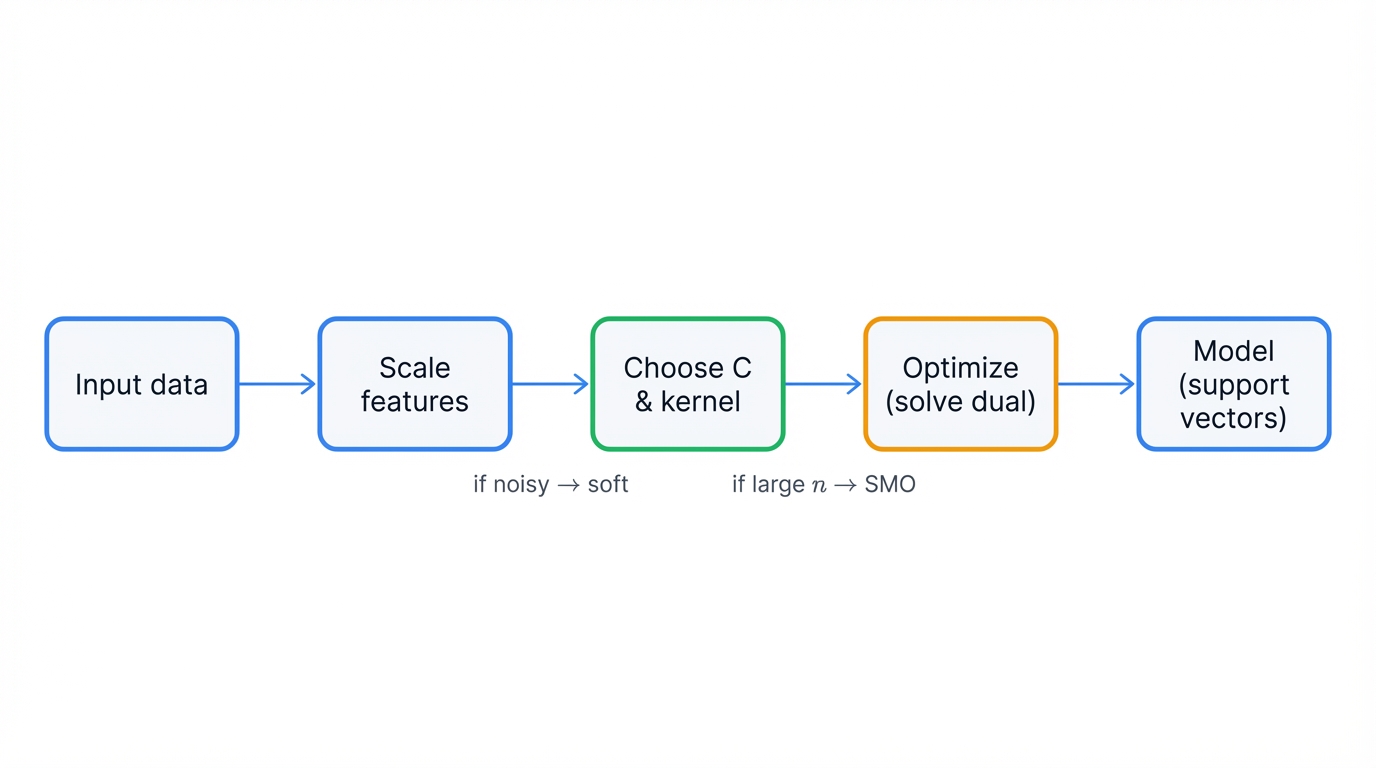
Data Preparation and Preprocessing begins with loading the labeled dataset. Separating features (X) from target labels (y). Binary classification conventionally uses -1 and +1 encoding for mathematical convenience. The most critical preprocessing step? Scaling feature data. Why? SVMs' distance-based margin calculations make them extremely sensitive to feature scale differences. Requiring mandatory scaling transformations such as StandardScaler to achieve zero mean and unit variance across all features.
Kernel and Hyperparameter Selection requires practitioners to choose kernel functions that determine the form of decision boundary the model can learn. Common choices? Linear kernels for simple separation. Polynomial kernels for moderate complexity. Radial Basis Function (RBF) kernels for highly non-linear problems. Initial hyperparameter values must be selected for the regularization parameter C and, for non-linear kernels, the kernel coefficient gamma. These values typically require optimization through systematic search procedures.
Solving the Dual Optimization Problem forms the computational core of SVM training. Through solving the dual quadratic programming problem derived from the mathematical formulation. The objective? Finding optimal Lagrange multiplier values (α_i) that maximize the dual objective function while satisfying all constraints. Modern implementations use Sequential Minimal Optimization (SMO). An efficient iterative algorithm that breaks the large quadratic programming problem into series of two-variable sub-problems that can be solved analytically. Dramatically accelerating the overall optimization process.
Identifying Support Vectors occurs after optimization convergence. The algorithm identifies training data points with non-zero optimal Lagrange multipliers (α_i > 0). These critical points lie exactly on or within the margin boundaries. Uniquely determine the optimal hyperplane. All other training points have zero influence on the final decision boundary.
Computing Model Parameters involves calculating the weight vector w and bias term b that define the optimal hyperplane. For linear SVMs, the weight vector is computed as a weighted sum of support vectors. The bias term is calculated using support vectors that lie exactly on the margin boundary. For kernel-based SVMs, explicit weight vector computation in the original feature space becomes impossible due to potentially infinite dimensionality. So the decision function remains in dual form using kernel evaluations.
Constructing the Final Decision Function creates the trained model used for making predictions on new data. Through either explicit weight vector computation for linear SVMs. Or dual-form kernel evaluation for non-linear SVMs.
For linear SVMs, the function is: $f(\mathbf{x}) = \text{sign}(\mathbf{w}^T\mathbf{x} + b)$.
For kernel SVMs, the function is expressed using the kernel trick. Summing only over the support vectors: $f(\mathbf{x}) = \text{sign}\left(\sum_{i \in SV} \alpha_i y_i K(\mathbf{x}_i, \mathbf{x}) + b\right)$.
Key Parameters: The Dials of Performance
The performance of an SVM? Critically dependent on the choice of its hyperparameters. Understanding how to tune these "dials" is essential for practical success.
kernel: This parameter specifies the kernel function. Which transforms the data into a feature space where a linear separation is sought. The choice of kernel is a form of injecting a prior assumption about the geometry of the data.
- linear: $K(\mathbf{x}_i, \mathbf{x}_j) = \mathbf{x}_i^T \mathbf{x}_j$. Assumes the data is linearly separable. Fastest and most interpretable option.
- poly: $K(\mathbf{x}_i, \mathbf{x}_j) = (\gamma \mathbf{x}_i^T \mathbf{x}_j + r)^d$. Creates a polynomial decision boundary. Requires tuning the degree (d).
- rbf (Radial Basis Function): $K(\mathbf{x}_i, \mathbf{x}_j) = \exp(-\gamma |\mathbf{x}_i - \mathbf{x}_j|^2)$. Most popular and flexible kernel. Can model complex, non-linear relationships. Often the default choice when data structure is unknown. Decision boundary is based on localized influence of support vectors.
- sigmoid: $K(\mathbf{x}_i, \mathbf{x}_j) = \tanh(\gamma \mathbf{x}_i^T \mathbf{x}_j + r)$. Inspired by neural networks. Used less in practice. RBF often provides superior results.
C (Regularization Parameter): This parameter controls the penalty for misclassification in the soft-margin formulation. Thereby managing the bias-variance trade-off.
- Low C: A smaller penalty for misclassified points. The optimization will favor a larger margin. Even if it means misclassifying more training points. This leads to a simpler, more generalized model (higher bias, lower variance) that is less sensitive to noise.
- High C: A large penalty for misclassification. The model will try to classify every training point correctly. Can result in a narrower margin. A more complex decision boundary that may overfit the training data (lower bias, higher variance).
gamma (Kernel Coefficient for rbf, poly, sigmoid): This parameter defines the scope of influence of a single training example. Can be seen as the inverse of the radius of influence of the support vectors.
- Low gamma: A single training example has far-reaching influence. The decision boundary will be very smooth and general. Behaving more like a linear model. This can lead to underfitting as the model is too constrained to capture the complexity of the data.
- High gamma: The influence of each support vector is very localized. The decision boundary can become highly irregular and "wiggly." Contouring closely to individual data points. This can lead to overfitting. As the model is essentially memorizing the training data, including its noise.
degree: Used only by the poly kernel. This parameter specifies the degree of the polynomial function. A higher degree allows for a more flexible and complex decision boundary. But also increases the risk of overfitting.
epsilon (for SVR): In the context of Support Vector Regression, epsilon (ε) defines the width of the margin of tolerance. Or "tube," around the regression function. Data points falling within this tube are not penalized. Making the model insensitive to errors smaller than ε.
The gamma and C hyperparameters should not be considered in isolation. Their interaction is crucial for defining the model's complexity. For instance, a very high gamma value can cause the model to overfit. Regardless of the C value. As the influence of each support vector becomes extremely localized. Conversely, with a very low gamma, the model becomes nearly linear. The C parameter's role in penalizing misclassifications becomes more pronounced. This means optimal performance is often found along a diagonal in the C-gamma parameter space. Where a smoother model (lower gamma) might require a higher penalty for errors (larger C) to become sufficiently complex. And vice versa. Therefore, any hyperparameter tuning strategy must explore their joint effect. Rather than tuning them independently.
The Training Process: Learning from Data
The SVM "learns" by solving the convex optimization problem defined by its objective function and constraints. Unlike many machine learning algorithms that use iterative methods like gradient descent, the SVM training process is deterministic. Given the same data and hyperparameters, it will always converge to the same unique, global optimal solution. This is a significant advantage over methods like neural networks. Which can be sensitive to initial conditions. May get trapped in local minima. The core of the training? The QP solver (like SMO). Which systematically adjusts the Lagrange multipliers (α_i) until the KKT optimality conditions are satisfied and the dual objective function is maximized. The result of this process? The set of support vectors and their corresponding weights. Which together define the maximal margin hyperplane.
Problem-Solving Capabilities
This section details the practical applications of Support Vector Machines. Showcasing the types of problems where the algorithm excels. Providing concrete examples of its successful deployment across various domains.
Primary Use Cases
SVMs are versatile algorithms. Can be adapted to several machine learning tasks. Though they are most famous for classification.
Binary Classification represents SVMs' native and most fundamental application. The algorithm designed specifically to find optimal hyperplanes that separate data into two distinct classes through geometric margin maximization. Classic examples? Spam versus legitimate email detection. Malignant versus benign tumor classification. Fraud versus legitimate transaction identification.
Multi-Class Classification extends SVM capabilities to problems with more than two classes. Through systematic decomposition strategies. Since SVMs are inherently binary classifiers. One-vs-Rest (OvR) strategy trains N separate binary classifiers for N-class problems. Each classifier distinguishes one specific class from all other classes combined. Then selecting the class with highest confidence score for final predictions. One-vs-One (OvO) strategy constructs binary classifiers for every possible pair of classes. Resulting in N(N-1)/2 classifiers for N-class problems. New data points classified through majority voting across all pairwise comparisons.
Regression through Support Vector Regression (SVR) adapts the SVM framework for predicting continuous numerical values. Rather than discrete class labels. This powerful variant uses epsilon-insensitive loss functions to create tolerance tubes around regression hyperplanes. Making SVR effective for forecasting, value estimation, and other regression tasks. While maintaining SVM's robustness advantages.
Outlier and Anomaly Detection through One-Class SVM represents an unsupervised application. Algorithms train on datasets containing only "normal" instances to learn boundary encapsulation of typical data patterns. New points falling outside these learned boundaries are flagged as anomalies or outliers. Making this approach valuable for fraud detection, network intrusion detection, and quality control applications where normal behavior can be characterized. But anomalies are rare or undefined.
Specific Examples and Success Stories
SVMs have been successfully applied in numerous fields. Particularly those characterized by high-dimensional data.
Bioinformatics: This is a domain where SVMs have had profound impact. Primarily due to their ability to handle datasets with a very large number of features (e.g., genes) and a relatively small number of samples (e.g., patients).
- Gene Expression and Cancer Classification: SVMs are used to analyze microarray data. To differentiate between cancerous and healthy tissue samples. Or to classify different subtypes of cancer based on gene expression patterns. Studies have reported accuracies as high as 90% in classifying breast cancer subtypes.
- Protein Classification and Remote Homology Detection: The algorithm is used to classify proteins into functional families based on their sequence or structural features. And to identify distant evolutionary relationships that are not easily detectable by sequence alignment methods alone.
- Disease Diagnosis: SVMs have been applied to predict the likelihood of diseases such as Alzheimer's. By analyzing genomic data. Achieving high accuracy. One biotech startup successfully used an SVM model to improve the accuracy of diagnostic tests for a rare genetic disorder. Reducing the rate of false positives by 30%.
Image Recognition: Before the widespread adoption of deep learning, SVMs were state-of-the-art for many computer vision tasks.
- Handwritten Digit Recognition: A classic benchmark problem in machine learning. Where SVMs have demonstrated excellent performance.
- Face Detection: SVMs can be trained to classify regions of an image as either containing a face or not. Forming a core component of face detection systems. Early versions of Facebook's photo tagging feature utilized SVMs for this purpose.
- Medical Image Analysis: In healthcare, SVMs are used to classify medical images. Such as identifying malignant tumors in MRI scans with high accuracy (AUC of 0.91 in one study). Or classifying skin lesions from dermoscopic images with 95% accuracy.
Text and Hypertext Categorization: SVMs are exceptionally well-suited for text classification. When text is converted into a numerical representation like TF-IDF, the resulting feature space is typically very high-dimensional and sparse. A scenario where SVMs excel.
- Spam Detection: A canonical binary classification task. Where SVMs are highly effective at distinguishing spam emails from legitimate ones.
- Sentiment Analysis: Classifying text (e.g., product reviews, social media comments) as expressing positive, negative, or neutral sentiment.
- Topic Classification: Automatically assigning documents, such as news articles or web pages, to predefined categories like 'sports', 'politics', or 'technology'.
Financial Applications:
- Fraud Detection: SVMs, particularly One-Class SVMs, are used to identify fraudulent credit card transactions. By modeling normal transaction behavior and flagging deviations as anomalies. One fintech company reported achieving a 95% accuracy rate in detecting fraudulent activities with an SVM-based system.
- Credit Scoring and Stock Market Prediction: The algorithm is also used for credit scoring. And to forecast financial trends. Such as predicting the direction of stock price movements.
The success of SVMs in bioinformatics and text classification is a direct consequence of the algorithm's core design. Its strength in high-dimensional spaces, where the number of features can dwarf the number of samples, is not an accidental benefit. It stems from the principle of margin maximization. Which is rooted in VC theory. Acts as a powerful form of regularization. Preventing the model from overfitting in these challenging "p > n" scenarios. This theoretical property translates directly into practical success in these specific domains.
Output Types
The nature of the output from an SVM model depends on the task it is configured to perform.
- Classification: The primary output is a discrete class label (e.g., -1 or +1). The model can also provide the signed distance of a data point from the decision hyperplane. This distance can be interpreted as a measure of classification confidence. The further a point is from the hyperplane, the more confident the prediction.
- Regression: The output is a single continuous numerical value. Representing the model's prediction for the given input.
- Anomaly Detection: The output is a binary label. Typically +1 for an "inlier" (normal data point) and -1 for an "outlier" (anomaly).
Performance Characteristics: When it Shines vs. When it Fails
Understanding the conditions under which SVMs thrive or struggle? Crucial for their effective application.
Scenarios of Strong Performance
- High-Dimensional Spaces: SVMs are particularly effective when the number of features is large. Even greater than the number of samples (p > n).
- Clear Margin of Separation: The algorithm excels when a clear, even if non-linear, boundary exists between the classes.
- Small to Medium-Sized Datasets: SVMs are a powerful choice for datasets where the number of samples is not prohibitively large. Allowing their robust optimization process to find high-quality solutions.
- Complex, Non-Linear Problems: Through the use of powerful kernels like the RBF kernel, SVMs can effectively model highly complex decision boundaries. Without requiring manual feature engineering.
Scenarios of Weak Performance
- Very Large Datasets: The quadratic to cubic training time complexity makes standard kernelized SVMs computationally infeasible for datasets with hundreds of thousands or millions of samples.
- Noisy Datasets with Overlapping Classes: When the classes have a large degree of overlap and the data is noisy, the concept of a clean, wide margin breaks down. The SVM may struggle to find a good separating hyperplane.
- Need for Probability Estimates: Standard SVMs do not provide direct probability estimates for class membership. While methods like Platt scaling can be used to calibrate them, this process is computationally expensive. The resulting probabilities may be inconsistent with the classifier's direct output.
- High Interpretability is Required: The decision-making process of a non-linear SVM is a "black box." Very difficult to interpret the model. Understand the contribution of individual features to a prediction.
Strengths and Limitations
Important Consideration: While this approach offers significant benefits, it's crucial to understand its limitations and potential challenges as outlined in this section.
This section provides a balanced and critical assessment of Support Vector Machines. Summarizing their key advantages and disadvantages. The underlying assumptions they make about the data. And their robustness to common real-world data imperfections.
Advantages: What Makes SVM Powerful?
The enduring popularity of SVMs can be attributed to a unique combination of theoretical elegance and practical effectiveness.
Effectiveness in High-Dimensional Spaces makes SVMs exceptionally powerful for complex problems like text classification and bioinformatics. Where feature counts often exceed sample counts (p > n). This capability stems from SVMs' margin maximization principle. That provides effective regularization in high-dimensional spaces. Preventing the overfitting that commonly affects other algorithms in similar scenarios.
Memory Efficiency emerges from SVMs' sparse solution property. The final decision function depends only on support vectors. Rather than the entire training dataset. This sparsity makes trained models remarkably compact and memory-efficient for prediction. Often requiring storage for only a small fraction of the original training data. While maintaining full decision-making capability.
Robustness to Overfitting derives from SVMs' implementation of Structural Risk Minimization through margin maximization. Providing strong regularization. Making models less prone to overfitting compared to complex alternatives like unregularized decision trees or neural networks. This theoretical foundation ensures reliable generalization. Even on challenging datasets with limited samples.
Versatility via Kernels represents SVMs' most powerful feature. Through the kernel trick. Enabling modeling of highly complex, non-linear decision boundaries by implicitly mapping data into higher-dimensional spaces. This provides immense flexibility to adapt to diverse data structures. Without requiring explicit feature engineering. Essentially allowing linear algorithms to solve non-linear problems.
Guaranteed Global Optimum stems from SVMs' convex quadratic programming foundation. Ensures unique, globally optimal solutions for every training problem. This mathematical guarantee eliminates the local minima problems that affect neural network training. Providing consistent, reproducible results. Regardless of initialization or training procedure variations.
Disadvantages: What are its Main Weaknesses?
Despite their strengths, SVMs have several notable limitations that practitioners must consider.
High Computational Complexity represents SVMs' primary limitation. Poor scalability with training sample count. Training time complexity of at least O(n²) makes them impractical for very large datasets. This quadratic scaling creates fundamental barriers to big data applications. Requiring practitioners to consider alternative algorithms when sample counts reach hundreds of thousands or millions.
Sensitivity to Hyperparameters and Kernel Choice creates significant tuning challenges. SVM performance depends heavily on optimal selection of kernel functions and hyperparameter values. Particularly the regularization parameter C and kernel coefficient gamma. Finding optimal combinations typically requires extensive, computationally expensive hyperparameter tuning. Through systematic cross-validation procedures.
Lack of Direct Probability Outputs limits SVMs' applicability in scenarios requiring confidence estimates. Standard classifiers produce class predictions based on decision function signs. Rather than class membership probabilities. While post-processing techniques like Platt scaling can generate probability estimates, these procedures are computationally expensive. May produce imperfectly calibrated probabilities that don't accurately reflect true prediction confidence.
Poor Interpretability in Non-Linear Cases creates "black box" problems. Where kernel SVMs become difficult to explain. Despite linear SVMs' interpretability through feature weights. Non-linear kernel SVMs operate in high-dimensional, abstract feature spaces. Where decision boundaries are simple hyperplanes. But their projections into original input spaces become incredibly complex surfaces. Cannot be easily described or understood in terms of original features. Making it difficult to explain specific prediction reasoning.
Performance Degradation on Noisy Data occurs when datasets contain significant noise and class overlap. That undermines SVMs' fundamental assumption of clean, wide margins separating distinct classes. In these scenarios, the core geometric optimization principles break down. Leading to substantial performance degradation compared to algorithms designed to handle noisy, overlapping distributions.
The "black box" problem is a direct and unavoidable trade-off for the power of the kernel trick. The very mechanism that makes SVMs so effective for non-linear problems is precisely what makes them so difficult to interpret. The kernel trick operates by implicitly mapping data to a space that could be infinite-dimensional. While the decision boundary is a simple hyperplane in this abstract space, its projection back into the original feature space becomes a highly complex, non-linear surface. Cannot be easily visualized or described by a simple set of rules. The model's parameters, the α_i values, correspond to the importance of the support vectors. Not the original features. Making it challenging to assess feature importance directly. This creates a fundamental choice for the practitioner: opt for a simple, interpretable linear model. Or leverage a kernel to obtain a powerful, non-linear, but uninterpretable model.
Assumptions of the Algorithm
Like all machine learning models, SVMs operate on a set of underlying assumptions about the data and the problem.
Linear Separability or Kernel-Transformable Separability forms SVMs' fundamental assumption. That data is, or can be made, linearly separable through appropriate transformations. Linear SVMs assume that a hyperplane can effectively separate classes in the original feature space. While kernel SVMs assume that appropriate mappings exist to higher-dimensional spaces where linear separation becomes possible. Enabling the algorithm's geometric optimization principles to find meaningful decision boundaries.
Independent and Identically Distributed (IID) Data represents a critical assumption shared with most statistical learning methods. Requiring that training data samples be drawn independently from identical underlying distributions. This assumption proves crucial for theoretical generalization guarantees to hold. Ensuring that patterns learned from training data will transfer effectively to unseen test data from the same distribution.
Fully Labeled Training Data reflects SVMs' supervised learning nature. Requiring that all training data points are accurately and completely labeled with correct class assignments. This complete labeling requirement enables the algorithm to learn optimal decision boundaries through the contrast between labeled examples. Making label quality and accuracy essential for effective model training.
Robustness to Data Imperfections
The practical utility of an algorithm often depends on how well it handles imperfect, real-world data.
Noise and Outliers are addressed through soft-margin SVMs' explicit robustness design. That introduces slack variables and regularization parameter C to handle anomalous points while finding generalizable decision boundaries. The algorithm can ignore some outliers to avoid overly complex boundaries. Though this robustness has limits. Outliers near decision boundaries can still become support vectors and influence final hyperplanes. Particularly with high C values that heavily penalize misclassification. Recent research continues developing more robust SVM formulations. That better handle extreme outlier scenarios.
Missing Data requires preprocessing attention. SVMs lack built-in mechanisms for handling incomplete feature matrices. Missing values must be addressed through imputation techniques before training. Though SVMs demonstrate interesting inherent robustness to missing data post-imputation. Since final model structure depends only on support vectors, missingness in non-support-vector data points may have minimal impact on classifier performance. Provided imputation procedures don't artificially transform missing-data points into support vectors.
Imbalanced Data can cause standard SVMs to perform poorly. Optimization may favor majority classes to minimize overall error. Creating decision boundaries that inadequately classify minority classes. This challenge can be mitigated through class weight adjustments (such as scikit-learn's class_weight='balanced'). That effectively increase misclassification penalties for minority classes. Rebalancing the optimization to achieve more equitable performance across all classes.
Distribution Shifts affect SVMs like most batch-trained machine learning models. That assume test data comes from the same distribution as training data. When underlying data distributions change over time—a common challenge in real-world applications—trained SVM model performance typically degrades. Requiring retraining or adaptation strategies to maintain effectiveness.
Comparative Analysis
This section positions Support Vector Machines within the broader landscape of machine learning classifiers. A detailed, head-to-head comparison with key alternatives is provided to guide practitioners. On when to choose one method over another. Highlighting the specific trade-offs involved.
Similar Methods
SVMs are part of a rich family of supervised learning algorithms. Each with its own strengths and weaknesses. The most common alternatives for classification tasks include:
Logistic Regression: A fundamental linear model widely used for binary classification. It works by modeling the probability of an instance belonging to a particular class. Using the logistic (sigmoid) function.
Decision Trees and Ensemble Methods (Random Forests, Gradient Boosting): These are non-parametric models that learn a hierarchy of simple, axis-aligned rules to partition the feature space. Ensemble methods like Random Forests combine many decision trees. To improve robustness and accuracy.
Artificial Neural Networks (ANNs) / Deep Learning: This broad class of models, inspired by the structure of the human brain, consists of interconnected layers of nodes (neurons). They are capable of learning extremely complex, hierarchical patterns and representations directly from data. They form the foundation of modern deep learning.
k-Nearest Neighbors (k-NN): A simple, instance-based learning algorithm that classifies a new data point based on the majority class of its k closest neighbors in the feature space. It makes no assumptions about the underlying data distribution.
When to Choose SVM over Alternatives
The decision to use an SVM should be based on the characteristics of the dataset. And the specific goals of the project.
vs. Logistic Regression (LR)
The core philosophical difference between SVM and Logistic Regression? One of geometry versus probability. SVM's objective is to find a geometric maximum margin. Its hinge loss function focuses exclusively on the boundary cases (the support vectors). In contrast, Logistic Regression's objective is to maximize the likelihood of the data under a probabilistic model. Its log loss function considers the contribution of every data point. This fundamental distinction explains nearly all of their practical differences.
Choose SVM when your problem characteristics align with the algorithm's strengths and theoretical advantages. High-dimensional data scenarios, especially when feature count exceeds sample count (p > n), leverage SVM's regularization through margin maximization. Proves particularly effective in preventing overfitting. Non-linear decision boundaries benefit from SVMs' kernel trick capabilities. Providing powerful, elegant approaches to capturing complex relationships that linear models cannot represent. Small to medium-sized datasets allow SVMs' computational requirements to remain manageable. While enabling their strong theoretical guarantees to prevent overfitting effectively. Robustness to outliers becomes important when SVM's margin-focused approach makes it less sensitive to extreme points. Compared to algorithms that consider all data points equally.
Choose Logistic Regression when your requirements prioritize interpretability, probability outputs, or large-scale performance. Over SVM's geometric optimization advantages. Model interpretability demands often favor logistic regression. Because its coefficients provide direct, understandable measures of feature importance. And their effects on outcomes. Probability outputs prove essential for many business applications like risk scoring. Where well-calibrated class probabilities enable confidence-based decision-making. Very large datasets favor logistic regression's superior computational efficiency. And scalability to large sample counts. Known linear separability scenarios allow logistic regression to provide simple, fast, and effective solutions. Without SVM's additional complexity.
vs. Decision Trees / Random Forests (DT/RF)
Choose SVM when your data characteristics favor geometric optimization over rule-based partitioning. High-dimensional and sparse data, particularly in text classification applications, often sees SVMs outperforming tree-based methods. Due to their effectiveness in high-dimensional spaces. Complex decision boundaries that aren't necessarily axis-aligned benefit from SVMs' ability to find optimal hyperplanes at any orientation. While decision trees are constrained to making splits perpendicular to feature axes. Limiting their flexibility for diagonal or curved boundaries.
Choose Decision Trees and Random Forests when interpretability and data handling flexibility take priority over geometric optimization. Interpretability requirements favor decision trees. Since their logic can be visualized as intuitive flowcharts of rules that stakeholders can easily understand and validate. Mixed numerical and categorical features are handled naturally by tree-based models. Without requiring extensive preprocessing like one-hot encoding that SVMs need. Feature scaling constraints favor trees. Since they're invariant to monotonic feature transformations. Eliminating SVM's mandatory scaling requirements. Large datasets generally favor Random Forests. Due to their faster training times compared to kernelized SVMs. And their natural parallelization capabilities.
vs. Neural Networks (NNs)
Choose SVM when dataset size and structure favor geometric optimization over deep feature learning. Small or medium-sized datasets benefit from SVMs' resistance to overfitting. Through their strong theoretical foundation in Structural Risk Minimization. Typically requiring fewer hyperparameter adjustments than deep neural networks. While providing superior generalization guarantees. Structured or tabular data with meaningful pre-existing features allows SVMs to serve as powerful baseline models. Or even achieve best-in-class performance. Without requiring the feature extraction capabilities that neural networks provide.
Choose Neural Networks when data scale or structure demands automatic feature learning and hierarchical pattern recognition. Very large datasets (millions of samples) favor neural networks' superior scalability characteristics. Compared to SVMs' quadratic complexity scaling. Raw, unstructured data such as image pixels, audio waveforms, or text characters requires the hierarchical feature learning capabilities. That represent deep neural networks' primary advantage over geometric methods. Extremely complex and hierarchical underlying relationships demand the flexible, expressive model architectures. That neural networks provide through their multi-layer, non-linear transformations.
Performance Trade-offs
The choice of algorithm involves balancing several competing factors. The following table provides a comparative summary of these trade-offs.
| Characteristic | Linear SVM | Kernel SVM | Logistic Regression | Random Forest | Neural Network |
|---|---|---|---|---|---|
| Model Type | Linear, Geometric | Non-Linear, Geometric | Linear, Probabilistic | Non-Linear, Ensemble | Non-Linear, Hierarchical |
| Interpretability | High (Feature Weights) | Low (Black Box) | High (Feature Coefficients) | Medium (Feature Importances) | Low (Black Box) |
| Scalability (Samples) | High | Low (O(n²)−O(n³)) | High | Medium to High | Very High |
| Scalability (Features) | High | High | Medium (can struggle with p>>n) | High | High |
| Non-Linearity | No | Yes (via Kernels) | No (requires manual features) | Yes (natively) | Yes (natively) |
| Data Scaling Req. | Required | Required | Recommended | Not Required | Required |
| Output Type | Class Label, Margin Distance | Class Label, Margin Distance | Class Probabilities | Class Probabilities | Class Probabilities |
| Key Strength | Speed, High-dim data | High accuracy on complex, medium data | Interpretability, Probabilities | Robustness, Ease of Use | Feature Learning, Scalability |
In the modern machine learning toolkit, the role of SVMs has evolved. Before the deep learning revolution, a well-tuned kernel SVM was often the algorithm of choice for achieving state-of-the-art performance on a wide range of tasks. Today, for unstructured data like images and audio, deep neural networks are dominant. However, for structured, tabular data of small-to-medium size, an SVM remains an extremely strong baseline model. Should not be overlooked. Numerous empirical studies and practitioner reports show that a well-tuned SVM can still be highly competitive with, and sometimes superior to, more modern ensemble methods like gradient boosting. Therefore, in a contemporary machine learning workflow for structured data, SVMs should be evaluated alongside tree-based ensembles and neural networks. As a primary candidate for the best-performing model.
Advanced Considerations
This section explores more advanced topics and extensions of the Support Vector Machine algorithm. Moving beyond standard binary classification. To address challenges in interpretability and scalability. Examining its application in regression, anomaly detection, and unsupervised learning.
Interpretability: The "Black Box" Problem
The interpretability of an SVM model varies dramatically depending on the kernel used.
Linear SVM: A linear SVM is a highly interpretable model. The trained weight vector, $\mathbf{w}$, contains coefficients that correspond directly to each input feature. The magnitude of a coefficient indicates the importance of that feature. In determining the position of the decision hyperplane. Its sign indicates its contribution towards one class or the other. This is analogous to the interpretability of coefficients in linear or logistic regression.
Kernel SVM: In stark contrast, a non-linear SVM using a kernel (like RBF) is notoriously difficult to interpret. Often referred to as a "black box" model. The decision is made in an abstract, high-dimensional, or even infinite-dimensional feature space. While the decision boundary is a simple hyperplane in that space, its projection back into the original, low-dimensional feature space is a complex, non-linear surface. Cannot be easily described or visualized. The model's parameters (α_i) relate to the support vectors, not the original features. Making it challenging to assess feature importance directly.
Techniques for Interpretation: To address this limitation, several techniques have been developed. Early methods included using permutation tests on feature weights to assess their significance. More recent research has focused on generating counterfactual explanations. This approach aims to answer the question: "What is the smallest change I can make to an input instance to flip the model's prediction to a different class?" By providing such concrete examples, these methods can make the SVM's decisions more tangible and understandable to a human user. This is an active area of research. Aimed at increasing the transparency and trustworthiness of SVM models.
Scalability: The Achilles' Heel
As previously discussed, the primary limitation of kernelized SVMs? Poor scalability with respect to the number of training samples (n). The quadratic to cubic training complexity is a major barrier to their use in "big data" applications.
The Bottleneck: The core issue? The need to solve a quadratic programming problem that, in its dual form, depends on the n × n kernel matrix. Both computing and storing this matrix become infeasible. As n grows into the hundreds of thousands or millions.
Mitigation Strategies:
- Use Linear SVMs: For very large datasets, if the problem is likely to be linearly separable in the high-dimensional feature space, using a highly optimized linear solver is the best approach. Implementations like LinearSVC in scikit-learn, which is based on the LIBLINEAR library, are orders of magnitude faster than kernelized SVMs.
- Stochastic Gradient Descent (SGD): An alternative way to train a linear SVM is to use stochastic gradient descent. The SGDClassifier in scikit-learn, when configured with loss='hinge', provides a linear SVM that can be trained on datasets that are too large to fit in memory. While this approach is much more scalable, it is an approximation. May not find the exact maximum-margin solution.
- Approximation and Parallelization: Advanced research has explored methods to make kernel SVMs more scalable. Random Fourier Features is a technique that can approximate kernel functions. Allowing a linear SVM to be trained on these new features. Much faster. Other approaches, like the Cascade SVM, attempt to parallelize the training process by splitting the data into chunks. Training SVMs on each chunk. Then iteratively combining the resulting support vectors. Recent academic work continues to push this boundary. Designing nearly-linear time algorithms for specific types of structured SVM problems.
Variants and Extensions
The core concept of margin maximization has proven remarkably flexible. Leading to the development of several important SVM variants that extend its capabilities beyond classification.
Support Vector Regression (SVR)
SVR adapts the SVM framework to solve regression problems. Where the goal is to predict a continuous numerical value.
Mechanism: Instead of finding a hyperplane that maximizes the margin separating two classes, SVR aims to find a hyperplane that best fits the data. The key innovation? The ε-insensitive loss function. This defines a "tube" or margin of tolerance with a width of ε around the hyperplane. Data points that fall within this tube are considered to have zero error. For points that fall outside the tube, a penalty is incurred. Proportional to their distance from the tube's edge.
Objective: The SVR optimization problem simultaneously tries to make the function $f(\mathbf{x})$ as "flat" as possible (by minimizing $|\mathbf{w}|^2$). While ensuring that most data points lie within the ε-tube.
Advantages: This approach makes SVR robust to outliers. Points with small errors do not affect the model. By using kernels, SVR can effectively capture complex, non-linear relationships in the data. A significant advantage over standard linear regression.
One-Class SVM
One-Class SVM is an unsupervised learning algorithm. Primarily used for anomaly detection or novelty detection.
Mechanism: It is trained on a dataset assumed to contain only "normal" or "inlier" data. The algorithm learns a boundary that encloses the majority of these normal data points. The objective is reframed to find a hyperplane that separates the data points from the origin in the feature space with maximum margin. This creates a tight boundary or hypersphere around the dense region of normal data.
Prediction: When a new data point is presented, the model determines whether it falls inside or outside this learned boundary. Points that fall outside are classified as anomalies or novelties.
Hyperparameter nu (ν): A key hyperparameter in One-Class SVM is ν. Which has a dual interpretation: it serves as an upper bound on the fraction of training points that can be considered outliers (margin errors). And a lower bound on the fraction of training points that must be support vectors.
Support Vector Clustering (SVC)
This is another unsupervised extension of the SVM framework. Designed to perform data clustering.
Mechanism: The algorithm first maps the data points to a high-dimensional feature space using a Gaussian kernel. In this space, it finds the smallest possible hypersphere that encloses the image of the data points. When this hypersphere is mapped back to the original data space, its boundary can form a set of disconnected, closed contours. Each distinct contour is then interpreted as a cluster boundary. All points enclosed by the same contour are assigned to the same cluster.
Properties: This method has the advantage of not requiring the number of clusters to be specified beforehand. Can identify clusters of arbitrary shapes and sizes. The width of the Gaussian kernel controls the scale and number of clusters detected.
The existence of this "family" of SVM algorithms demonstrates the remarkable flexibility of the core margin-maximization concept. The same fundamental optimization machinery—constrained quadratic programming, support vectors, and the kernel trick—can be adapted from supervised classification to regression, anomaly detection, and even clustering. Simply by reframing the objective function. This shows that the core SVM idea represents not just a single classification algorithm. But a powerful and generalizable framework for defining optimal boundaries in data.
Feature Engineering
While the kernel trick is a form of powerful, implicit feature engineering, explicit preparation of features can still significantly improve SVM performance.
Scaling: As emphasized throughout, scaling numerical features is a mandatory step.
Dimensionality Reduction: For datasets with an extremely large number of features, dimensionality reduction techniques like Principal Component Analysis (PCA) can be beneficial. PCA can help reduce computational costs. Remove noise. Mitigate multicollinearity by projecting the data onto a lower-dimensional subspace of principal components.
Domain-Specific Feature Creation: For specific tasks, manually engineering meaningful features can be more effective than relying solely on a generic kernel. For instance, in image recognition, using established feature descriptors like HOG or SIFT to capture shape and texture information before feeding them to an SVM can yield better performance. Than using raw pixel values. Similarly, for text, using sophisticated representations like TF-IDF or embeddings is crucial.
Practical Guidance
This section provides actionable advice for practitioners using SVMs. Focusing on best practices. Common mistakes to avoid. And systematic approaches for tuning and evaluation to achieve optimal performance.
Implementation Tips: Best Practices
Best Practice: Following these recommended practices will help you achieve optimal results and avoid common pitfalls.
Following a set of best practices is crucial for building effective and reliable SVM models.
Scale Your Data represents the most critical preprocessing step. Must be completed before SVM training. Due to the algorithm's fundamental reliance on distance metrics. That are highly sensitive to feature value ranges. Always apply scaling transformations such as StandardScaler. To achieve zero mean and unit variance. Ensuring that all features contribute appropriately to margin calculations. Rather than allowing large-scale features to dominate the geometric optimization process.
Start with Simple Kernels by beginning with linear kernels. That train significantly faster. May provide adequate performance for many problems. Eliminating the need for more complex alternatives. When linear kernels prove insufficient, the Radial Basis Function (RBF) kernel provides a powerful, flexible default choice for non-linear problems. That can capture complex decision boundaries. While maintaining reasonable computational requirements.
Handle Class Imbalance proactively. Standard SVMs may become biased toward majority classes in imbalanced datasets. Leading to poor minority class performance. Use scikit-learn's class_weight='balanced' parameter. To automatically adjust regularization parameter C inversely proportional to class frequency. Effectively increasing penalties for minority class misclassification. Achieving more balanced performance across all classes.
Use Proper Data Splitting by always partitioning datasets into separate training and testing sets. To obtain unbiased estimates of model performance on unseen data. Typical 80/20 training/testing splits provide good balance between training data volume and evaluation reliability. While k-fold cross-validation offers more robust evaluation approaches. Particularly valuable for smaller datasets.
Common Pitfalls and How to Avoid Them
Practitioners new to SVMs often encounter a few common mistakes. That can severely degrade model performance.
Forgetting to Scale Features represents the most frequent and impactful error. Leads to models where large-scale features dominate learning processes. Create suboptimal hyperplanes. Avoid this by integrating feature scaling as a standard, non-negotiable pipeline step. Preferably using tools like scikit-learn's Pipeline that prevent data leakage from test sets into scaler training. Ensure consistent preprocessing across all data splits.
Applying Kernel SVMs to Very Large Datasets creates prohibitive computational barriers. Training kernelized SVMs on millions of samples leads to excessive training times. Or memory errors due to O(n²) complexity scaling. Avoid this by assessing whether linear models suffice for large datasets. Using highly optimized LinearSVC or SGDClassifier with hinge loss for linear cases. Or considering data subsampling and alternative scalable algorithms like gradient boosting or neural networks. When non-linearity is essential.
Using Inappropriate Kernels results in poor performance. When linear kernels are applied to fundamentally non-linear decision boundaries. Since the model lacks capacity to capture underlying patterns. Avoid this through data visualization when possible to understand structural characteristics. Or pragmatically test both linear and RBF kernels. To compare cross-validated performance. Select the most appropriate approach.
Neglecting Hyperparameter Tuning leads to suboptimal results. Default library hyperparameters rarely provide best performance for specific problems. SVM performance being extremely sensitive to C and gamma parameter selections. Avoid this by always performing systematic hyperparameter search. Using validation sets or cross-validation. To identify optimal parameter combinations. That maximize performance for your particular dataset and problem requirements.
A systematic pipeline is non-negotiable for SVMs. The strong interdependencies between preprocessing (scaling), model selection (kernel choice), and optimization (hyperparameter tuning) mean that an ad-hoc or piecemeal approach is likely to fail. A successful SVM implementation is less about the isolated algorithm. More about the rigor of the end-to-end process surrounding it. For example, improper scaling leads to a meaningless hyperparameter search. Which in turn leads to a suboptimal model. Regardless of the kernel chosen. Therefore, practitioners should think in terms of a unified Pipeline. Where scaling and model fitting are bundled together. This ensures that during cross-validation and hyperparameter search, the entire process is evaluated correctly. Preventing data leakage. Leading to a truly generalizable model.
Hyperparameter Tuning Strategies
Finding the optimal hyperparameters? Key to unlocking the full potential of an SVM. Several systematic strategies exist for this search.
Grid Search (GridSearchCV) provides exhaustive, brute-force hyperparameter optimization. By defining discrete value grids for each parameter. Training models for every possible combination. While guaranteed to find optimal combinations within specified grids, computational costs grow exponentially with parameter count. Making this approach very slow for large search spaces. But reliable for small, well-defined parameter ranges.
Random Search (RandomizedSearchCV) offers more efficient optimization. By sampling fixed numbers of hyperparameter combinations from specified statistical distributions. Rather than exhaustively testing every combination. This approach operates on the principle that not all hyperparameters contribute equally to performance. Often finding very good or optimal combinations much faster than grid search. By exploring wider, more diverse value ranges.
Bayesian Optimization represents the most intelligent and efficient model-based optimization technique. That builds probabilistic surrogate models (typically Gaussian Processes) of relationships between hyperparameters and performance scores. This approach intelligently selects subsequent hyperparameter combinations. By balancing exploration of uncertain areas with exploitation of promising regions. Typically requiring far fewer evaluations than grid or random search. To achieve optimal parameters. Making it ideal when individual model training is computationally expensive.
The choice of tuning strategy reflects a trade-off between computational budget and optimization efficiency. With a small search space and ample time, Grid Search is simple and reliable. For a larger search space, Random Search is a more practical and often equally effective choice. When the cost of evaluating a single hyperparameter combination is very high (e.g., training a complex SVM on a large dataset), the additional complexity of Bayesian Optimization is justified. By its significant reduction in the total number of required training runs.
The following table provides a practical guide for tuning the key SVM hyperparameters.
| Hyperparameter | Role / Function | Effect on Model (Bias-Variance) | Typical Search Range / Values |
|---|---|---|---|
| kernel | Defines the transformation to the feature space and the shape of the decision boundary. | Controls the fundamental flexibility of the model. | ['linear', 'rbf']. Start with linear, then try rbf. poly is less common. |
| C | Regularization parameter. Controls the trade-off between margin width and training error. | Low C: Wider Margin, Higher Bias, Lower Variance (Underfitting). High C: Narrower Margin, Lower Bias, Higher Variance (Overfitting). | Logarithmic scale, e.g., [0.1, 1, 10, 100, 1000] |
| gamma | Kernel coefficient for rbf, poly, sigmoid. Defines the influence of a single training point. | Low gamma: Broad Influence, Smoother Boundary, Higher Bias, Lower Variance (Underfitting). High gamma: Local Influence, Complex Boundary, Lower Bias, Higher Variance (Overfitting). | Logarithmic scale, e.g., [1e-4, 1e-3, 0.01, 0.1, 1] |
| degree | Degree of the polynomial for the poly kernel. | Controls the flexibility of the polynomial decision boundary. Higher degree leads to a more complex model (higher variance). | Small integers, e.g., [2, 3, 4, 5] |
Appropriate Evaluation Metrics
Choosing the right metric to evaluate an SVM model? As important as training it correctly. The choice depends on the problem and the nature of the data.
Accuracy: The proportion of correctly classified instances. A good general-purpose metric. But can be very misleading on imbalanced datasets.
Precision, Recall, and F1-Score: These metrics are essential for imbalanced classification problems.
- Precision: Of all the instances the model predicted as positive, what fraction were actually positive? (TP / (TP + FP)). High precision is important when the cost of a false positive is high.
- Recall (Sensitivity): Of all the actual positive instances, what fraction did the model correctly identify? (TP / (TP + FN)). High recall is important when the cost of a false negative is high.
- F1-Score: The harmonic mean of precision and recall (2 · (Precision · Recall) / (Precision + Recall)). Provides a single score that balances both concerns.
Confusion Matrix: A table that provides a detailed breakdown of classification results. Showing the counts of True Positives (TP), True Negatives (TN), False Positives (FP), and False Negatives (FN). Invaluable for understanding the specific types of errors the model is making.
ROC Curve and AUC: The Receiver Operating Characteristic (ROC) curve is a plot of the True Positive Rate (Recall) against the False Positive Rate. For different classification thresholds. The Area Under the Curve (AUC) provides a single, aggregate measure of performance across all possible thresholds. An AUC of 1.0 represents a perfect classifier. While an AUC of 0.5 represents a model that is no better than random guessing.
Recent Developments
This final section brings the discussion of Support Vector Machines into the modern era. Exploring current research trends, future directions, and how the algorithm maintains its relevance. In an industry increasingly dominated by deep learning.
Current Research: Pushing the Boundaries
Despite being a mature algorithm, SVMs remain an active area of research. With a focus on addressing their primary limitations. Extending their capabilities.
Faster Algorithms and Scalability: A major thrust of current research? Overcome the scalability bottleneck of kernel SVMs. Researchers are developing more efficient solvers for the underlying quadratic programming problem. One promising direction involves designing algorithms with nearly-linear time complexity for specific structured problems. Such as when the data matrix has a low-rank factorization. Would represent a significant improvement over the standard quadratic or cubic complexity.
Enhanced Robustness: While the soft-margin SVM offers some robustness, researchers are developing new formulations. More explicitly designed to handle noise, outliers, and class imbalance. These models may, for example, modify the objective function to penalize the number of margin violations. Rather than their magnitude. Making the model less sensitive to extreme outliers.
Improved Interpretability: To combat the "black box" nature of kernel SVMs, research is underway to develop methods for explaining their predictions. A notable area? The generation of counterfactual explanations. Which identify the minimal changes to an input's features that would flip the model's prediction. This provides actionable insights into the model's decision-making process.
Quantum SVM (QSVM): At the cutting edge of computing, researchers are exploring quantum algorithms for machine learning. QSVM aims to leverage the principles of quantum mechanics. To potentially achieve exponential speedups in training time. The approach involves mapping feature vectors to a quantum state space. While still largely theoretical and reliant on the development of fault-tolerant quantum computers, current work uses GPU-accelerated quantum simulators. To test and develop these algorithms on real-world scientific datasets. Such as for large-scale stellar classification.
Future Directions: The Next Five Years
The evolution of SVMs is expected to continue. With a focus on integration, automation, and specialization.
Hybrid Models: A significant future direction? The deeper integration of SVMs with deep learning frameworks. Instead of being competing models, they can be complementary. SVMs can serve as a powerful, theoretically-grounded final classification layer. On top of the rich, hierarchical features extracted by a deep neural network. This hybrid approach can combine the feature-learning power of deep learning. With the margin-maximization principle of SVMs.
Advanced Kernel Development: Research continues into designing more sophisticated kernel functions. Tailored for specific types of complex data. Such as graphs, time series, or structured biological data. These custom kernels can better capture the inherent similarity and structure within these domains.
Automated Machine Learning (AutoML): The complex and crucial process of kernel selection, data preprocessing, and hyperparameter tuning for SVMs makes them a prime candidate for automation. Future AutoML systems will likely incorporate more sophisticated SVM tuning pipelines. Making the algorithm more accessible and easier to deploy optimally. Without deep expert knowledge.
Hardware Acceleration: Beyond quantum computing, ongoing efforts to accelerate SVM training on parallel hardware like GPUs will continue. Libraries that can leverage GPU power for the intensive matrix operations involved in kernel computation will make SVMs more viable for moderately large datasets.
Industry Trends and Modern Relevance
In an industry landscape increasingly dominated by deep learning, SVMs have carved out a durable and important niche.
A Powerful Baseline in Industry: While no longer the default choice for every problem, a well-tuned SVM remains a formidable baseline in many industrial applications. In sectors like manufacturing, SVMs are used for high-accuracy quality control and predictive maintenance. In finance, they are applied to risk assessment and fraud detection. Their robust performance on structured, medium-sized datasets makes them an essential benchmark. That more complex models must outperform.
Enduring Strength in Niche Domains: SVMs continue to be a leading method in fields where their unique strengths align with the data characteristics. This is especially true in bioinformatics and computational biology. Where high-dimensional genomic and proteomic data from a limited number of samples is the norm. SVMs are used to discover cancer biomarkers. Aid in drug discovery. Analyze complex genomic patterns.
The Surprising Connection to Transformers: A recent and profound theoretical development has established a formal equivalence. Between the self-attention mechanism at the heart of the Transformer architecture. And a hard-margin SVM problem. This research suggests that the attention layer can be interpreted as implicitly solving an SVM problem. To separate "optimal" input tokens from non-optimal ones. This finding provides a new theoretical lens for understanding one of today's most powerful deep learning models. Suggests that the core principles of margin maximization are more fundamental to machine learning than previously thought.
The trajectory of SVM research mirrors the evolution of the machine learning field itself. The initial focus on theoretical soundness (VC theory) and predictive power (kernels) has matured into a focus on addressing the practical engineering challenges. Of scalability, interpretability, and robustness. This reflects the broader shift of machine learning from a purely academic discipline. To a core engineering one. Where models must not only be accurate. But also efficient, trustworthy, and deployable in real-world systems.
Learning Resources
For those wishing to deepen their understanding of Support Vector Machines, a wealth of high-quality resources is available.
Essential Academic Papers
- Vapnik, V. N. (1995). The Nature of Statistical Learning Theory. The foundational text that details the statistical learning theory (including VC theory and SRM) upon which SVMs are built.
- Cortes, C., & Vapnik, V. (1995). "Support-vector networks." Machine Learning. The seminal paper that introduced the soft-margin formulation. Making SVMs practical for real-world, non-separable data.
- Boser, B. E., Guyon, I. M., & Vapnik, V. N. (1992). "A training algorithm for optimal margin classifiers." Proceedings of the Fifth Annual Workshop on Computational Learning Theory. The groundbreaking paper that first introduced the kernel trick. Enabling non-linear classification.
- Platt, J. C. (1999). "Fast training of support vector machines using sequential minimal optimization." In Advances in Kernel Methods: Support Vector Learning. This paper describes the SMO algorithm. The efficient optimization technique that made training SVMs practical. Used in major libraries like LIBSVM.
- Burges, C. J. (1998). "A tutorial on support vector machines for pattern recognition." Data Mining and Knowledge Discovery. A classic and highly-cited tutorial that provides a comprehensive mathematical and intuitive introduction to the topic.
Tutorials and Courses
- Online Courses: Platforms like Coursera, Udemy, and edX offer numerous machine learning courses. That provide detailed lectures and assignments on SVMs. Notable instructors include Andrew Ng and Pascal Poupart.
- Video Tutorials: Excellent intuitive explanations can be found on YouTube channels. Such as StatQuest with Josh Starmer, which breaks down the main ideas and Python implementation. And Krish Naik, who provides in-depth videos on specific concepts like kernels.
- Practical Guides: Websites like DataCamp, GeeksforGeeks, and Analytics Vidhya offer step-by-step tutorials with code. For implementing SVMs in Python using scikit-learn. Often using benchmark datasets like the Iris or breast cancer datasets for demonstration.
Code Examples and Repositories
GitHub: GitHub is an invaluable resource for practical examples. Searching for topics like svm-training, linear-svm, or simply svm reveals thousands of repositories. These range from simple Jupyter Notebook tutorials on benchmark datasets. To complex applications in fields like finance, computer vision, and natural language processing.
Key Repositories:
- cjlin1/libsvm: The official repository for the LIBSVM library. The foundational software for many SVM implementations.
- Scikit-learn Documentation: The official scikit-learn website provides extensive documentation. With clear code examples for all its SVM implementations (SVC, LinearSVC, SVR).
- Kaggle: Kaggle hosts numerous datasets and public notebooks (kernels). Where practitioners share their code and analysis using SVMs. For a wide variety of predictive modeling tasks.
Example Implementation
# Example: Model training with security considerations
import numpy as np
from sklearn.model_selection import train_test_split
from sklearn.ensemble import RandomForestClassifier

def train_secure_model(X, y, validate_inputs=True):
    """Train model with input validation"""

    if validate_inputs:
        # Validate input data
        assert X.shape[0] == y.shape[0], "Shape mismatch"
        assert not np.isnan(X).any(), "NaN values detected"

    # Split data securely
    X_train, X_test, y_train, y_test = train_test_split(
        X, y, test_size=0.2, random_state=42, stratify=y
    )

    # Train with secure parameters
    model = RandomForestClassifier(
        n_estimators=100,
        max_depth=10,  # Limit to prevent overfitting
        random_state=42
    )

    model.fit(X_train, y_train)
    score = model.score(X_test, y_test)

    return model, score