Watch a toddler learn to walk. Stumble. Fall. Try again. This is reinforcement learning in its purest form—no instruction manual, no labeled examples, just trial, error, and gradual mastery through direct experience with the world.
Reinforcement Learning powers the AI systems that beat world champions at Go, drive autonomous cars through chaotic city streets, and predict your next Netflix obsession with uncanny accuracy. Unlike supervised learning, which demands laboriously labeled training examples, or unsupervised learning, which quietly discovers hidden patterns in unlabeled data, RL learns through pure interaction—taking actions, receiving feedback, adapting strategy, and iterating relentlessly toward optimal performance.
The Learning Paradigm That Changed Everything
The Agent-Environment Dance: How RL Really Works
Think of it as a conversation. An endless, evolving dialogue between two entities locked in a feedback loop that never stops learning, never stops adapting, and never stops getting better at achieving its goals.
RL in Production
Reinforcement learning presents unique deployment challenges. Reward hacking, exploration risks, and safety constraints require careful consideration in production systems.
RL trains software agents to make optimal decisions through trial-and-error learning, creating an interactive feedback loop between two players locked in constant communication. The Agent is the learner—you, playing a video game, desperately trying to win. The Environment is the world itself—the game with all its ruthless rules, its unforgiving physics, its precise dynamics that care nothing for your intentions.
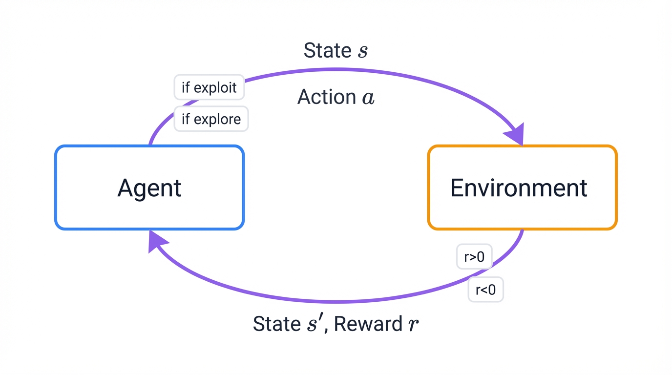
The interaction unfolds in discrete time steps, a rhythmic dance of observation and action. Each step follows an ironclad sequence that governs every RL system ever built.
RL Agent-Environment Interaction Loop
First, the agent observes. It examines the current state of the environment, gathering every scrap of available information about the situation it faces. Second, it acts—selecting one action from all available options based on its current understanding, its accumulated wisdom, its best guess about what will work. Third, the environment responds by transitioning to a new state based on the action taken, shifting the entire game board in response to the agent's choice. Finally, the environment delivers its verdict through a reward signal that can be positive, negative, or neutral, brutally honest feedback indicating how good or catastrophically bad that action turned out to be.
Picture a continuous cycle. Agent observes, then acts. Environment responds, agent observes the new state. Repeat. This observation-action-feedback loop drives every RL system ever deployed, from game-playing AI to warehouse robots to trading algorithms.
Here's the key insight that separates RL from simple reactive systems: agents don't chase immediate rewards like dogs chasing squirrels—they maximize cumulative long-term rewards across entire sequences of decisions, requiring strategic thinking, careful planning, and the discipline of delayed gratification that distinguishes intelligence from mere reflex.
Chess players sacrifice pieces for better board position. RL agents learn this same profound lesson—that sometimes short-term pain, temporary setbacks, and immediate losses lead inexorably to long-term gain, ultimate victory, and optimal outcomes that couldn't be achieved through greedy short-sighted decision-making. The agent develops a strategy called a policy that dictates which actions to take in which states to maximize expected future rewards, balancing immediate payoffs against long-term consequences in a delicate calculus of value and risk.
This demands balancing exploration with exploitation. Try new things or use what works? The eternal dilemma haunts every learning system.
Working Example: Reinforcement Learning Fundamentals - GridWorld
import numpy as np
import matplotlib.pyplot as plt
from collections import defaultdict

class GridWorld:
    def __init__(self, size=4):
        self.size = size
        self.state_space = size * size
        self.action_space = 4  # up, down, left, right
        self.actions = ['up', 'down', 'left', 'right']

        # Define goal and starting positions
        self.goal_state = (size-1, size-1)  # bottom-right corner
        self.start_state = (0, 0)  # top-left corner
        self.current_state = self.start_state

        # Define rewards
        self.goal_reward = 10
        self.step_penalty = -0.1
        self.wall_penalty = -1

    def reset(self):
        """Reset environment to starting state"""
        self.current_state = self.start_state
        return self.current_state

    def is_valid_state(self, state):
        """Check if state is within grid boundaries"""
        row, col = state
        return 0 <= row < self.size and 0 <= col < self.size

    def get_next_state(self, state, action):
        """Calculate next state given current state and action"""
        row, col = state

        if action == 0:  # up
            next_state = (row - 1, col)
        elif action == 1:  # down
            next_state = (row + 1, col)
        elif action == 2:  # left
            next_state = (row, col - 1)
        elif action == 3:  # right
            next_state = (row, col + 1)
        else:
            next_state = state

        # If next state is invalid, stay in current state
        if not self.is_valid_state(next_state):
            return state
        return next_state

    def step(self, action):
        """Take action and return next state, reward, and done flag"""
        next_state = self.get_next_state(self.current_state, action)

        # Calculate reward
        if next_state == self.current_state:  # hit wall
            reward = self.wall_penalty
        elif next_state == self.goal_state:  # reached goal
            reward = self.goal_reward
        else:  # normal step
            reward = self.step_penalty

        self.current_state = next_state
        done = (next_state == self.goal_state)

        return next_state, reward, done

class QLearningAgent:
    def __init__(self, state_space, action_space, learning_rate=0.1,
                 discount_factor=0.95, epsilon=1.0, epsilon_decay=0.995):
        self.state_space = state_space
        self.action_space = action_space
        self.learning_rate = learning_rate
        self.discount_factor = discount_factor
        self.epsilon = epsilon
        self.epsilon_decay = epsilon_decay
        self.epsilon_min = 0.01

        # Initialize Q-table
        self.q_table = defaultdict(lambda: np.zeros(action_space))

    def choose_action(self, state):
        """Choose action using epsilon-greedy policy"""
        if np.random.random() < self.epsilon:
            # Exploration: choose random action
            return np.random.choice(self.action_space)
        else:
            # Exploitation: choose best known action
            return np.argmax(self.q_table[state])

    def update_q_value(self, state, action, reward, next_state):
        """Update Q-value using Q-learning equation"""
        current_q = self.q_table[state][action]
        max_next_q = np.max(self.q_table[next_state])

        # Q-learning update rule
        new_q = current_q + self.learning_rate * (
            reward + self.discount_factor * max_next_q - current_q
        )

        self.q_table[state][action] = new_q

    def decay_epsilon(self):
        """Decay exploration rate"""
        if self.epsilon > self.epsilon_min:
            self.epsilon *= self.epsilon_decay

# Training the RL Agent
def train_agent(episodes=1000):
    env = GridWorld(size=4)
    agent = QLearningAgent(state_space=16, action_space=4)

    episode_rewards = []
    episode_steps = []

    for episode in range(episodes):
        state = env.reset()
        total_reward = 0
        steps = 0

        while True:
            action = agent.choose_action(state)
            next_state, reward, done = env.step(action)

            # Update Q-table
            agent.update_q_value(state, action, reward, next_state)

            state = next_state
            total_reward += reward
            steps += 1

            if done or steps > 100:  # prevent infinite loops
                break

        agent.decay_epsilon()
        episode_rewards.append(total_reward)
        episode_steps.append(steps)

        if episode % 100 == 0:
            avg_reward = np.mean(episode_rewards[-100:])
            print(f"Episode {episode}, Average Reward: {avg_reward:.2f}, Epsilon: {agent.epsilon:.3f}")

    return agent, episode_rewards, episode_steps

# Run training
print("Training Q-Learning Agent on GridWorld...")
trained_agent, rewards, steps = train_agent(episodes=1000)

# Test trained agent
def test_agent(agent, episodes=10):
    env = GridWorld(size=4)
    test_rewards = []

    # Turn off exploration for testing
    agent.epsilon = 0

    for episode in range(episodes):
        state = env.reset()
        total_reward = 0
        path = [state]

        while True:
            action = agent.choose_action(state)
            next_state, reward, done = env.step(action)

            state = next_state
            total_reward += reward
            path.append(state)

            if done or len(path) > 50:
                break

        test_rewards.append(total_reward)
        print(f"Test Episode {episode + 1}: Reward = {total_reward:.2f}, Steps = {len(path)-1}")
        print(f"Path taken: {path}")
        print()

    print(f"Average test reward: {np.mean(test_rewards):.2f}")

print("\nTesting trained agent...")
test_agent(trained_agent, episodes=5)
Watch this example bring RL to life. We build a simple GridWorld environment where an agent learns to navigate from start to goal through pure trial and error, accumulating wisdom through experience, discovering through countless failures that the shortest path yields the highest cumulative reward, and eventually mastering a task it initially approached with complete ignorance.
The agent starts knowing nothing. It fumbles, explores randomly, crashes into walls, takes circuitous routes that waste precious steps. But with each episode, each journey from start to goal, it learns. The Q-learning algorithm updates its understanding of action values, gradually building an internal map of what works and what doesn't, transforming random wandering into purposeful navigation that converges on optimal behavior.
The Mathematical Foundation of RL
Every successful RL system rests on solid mathematical foundations. Understanding these concepts transforms RL from mysterious black box into predictable engineering tool, from intimidating abstraction into concrete framework you can reason about, debug, and optimize with confidence.
Markov Decision Process: The Mathematical Framework
Every RL problem formalizes as a Markov Decision Process. No exceptions. This mathematical framework provides the theoretical foundation for all reinforcement learning algorithms, giving us a rigorous language to describe decision-making under uncertainty with precision, elegance, and the clarity that enables both theoretical analysis and practical implementation.
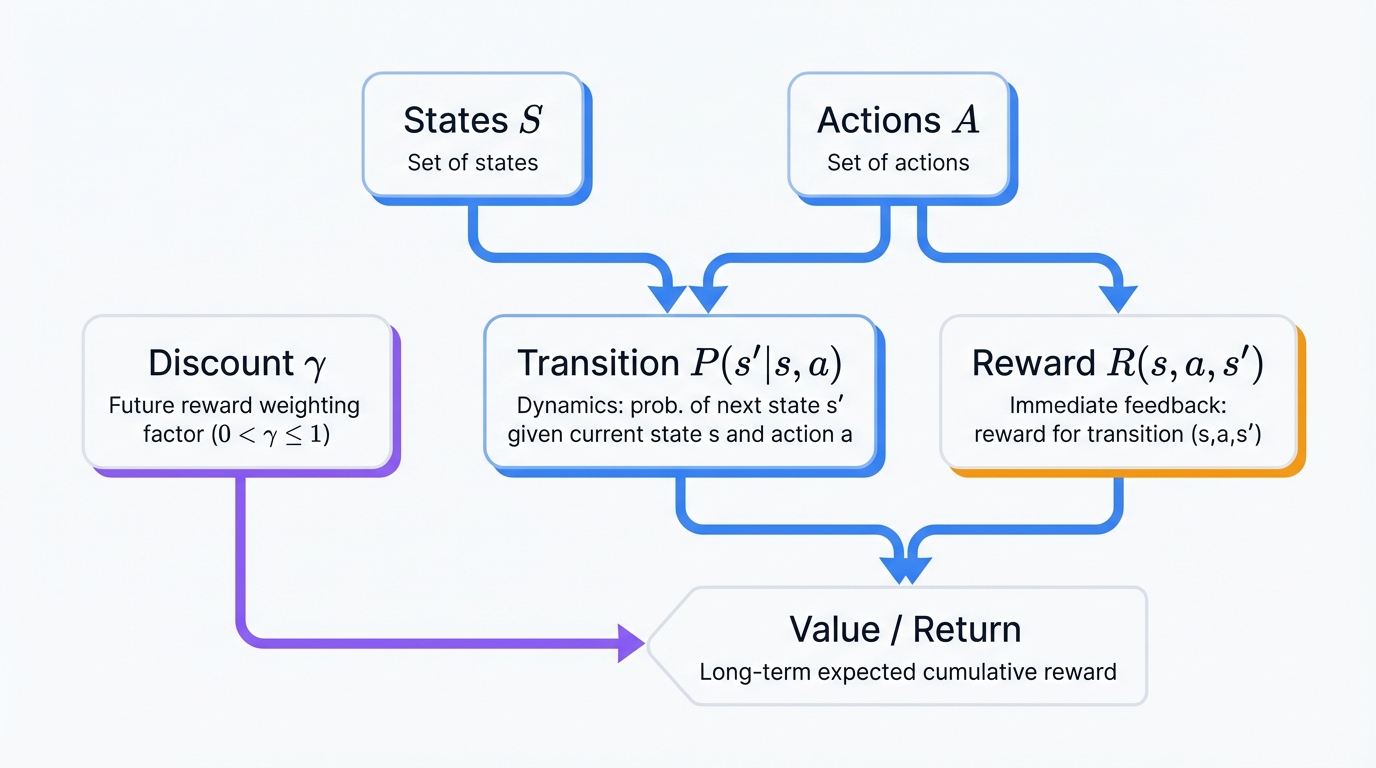
The MDP Components:
- States (S): All possible situations the agent can encounter in its world
- Actions (A): All possible moves the agent can execute from any state
- Transition Probabilities P(s'|s,a): Likelihood of reaching state s' from state s after taking action a
- Reward Function R(s,a,s'): Immediate reward received for transitioning from s to s' via action a
- Discount Factor γ: How much future rewards matter relative to immediate rewards (0 ≤ γ ≤ 1)
MDP Structure Visualization
The Markov Property: Here's the crucial assumption that makes everything work—the future depends only on the present state, not the entire history of how you arrived there. This "memoryless" property means you don't need to track every step you've ever taken to make optimal decisions, simplifying the mathematics dramatically, making problems tractable, and enabling the powerful algorithms we'll explore next.
Policy π(a|s): The agent's strategy. A mapping from states to actions. Finding the optimal policy π* is the ultimate goal of every RL algorithm ever designed.
Value Functions: Predicting Future Success
Value functions estimate how good situations are. They answer the critical question every agent faces: if I find myself in this state, or if I take this action from this state, how much cumulative reward can I expect to collect over the rest of this episode, and how do I use that prediction to make better decisions right now?
These functions sit at the center of most RL algorithms, providing the value estimates that guide exploration, drive learning, and ultimately converge to optimal policies.
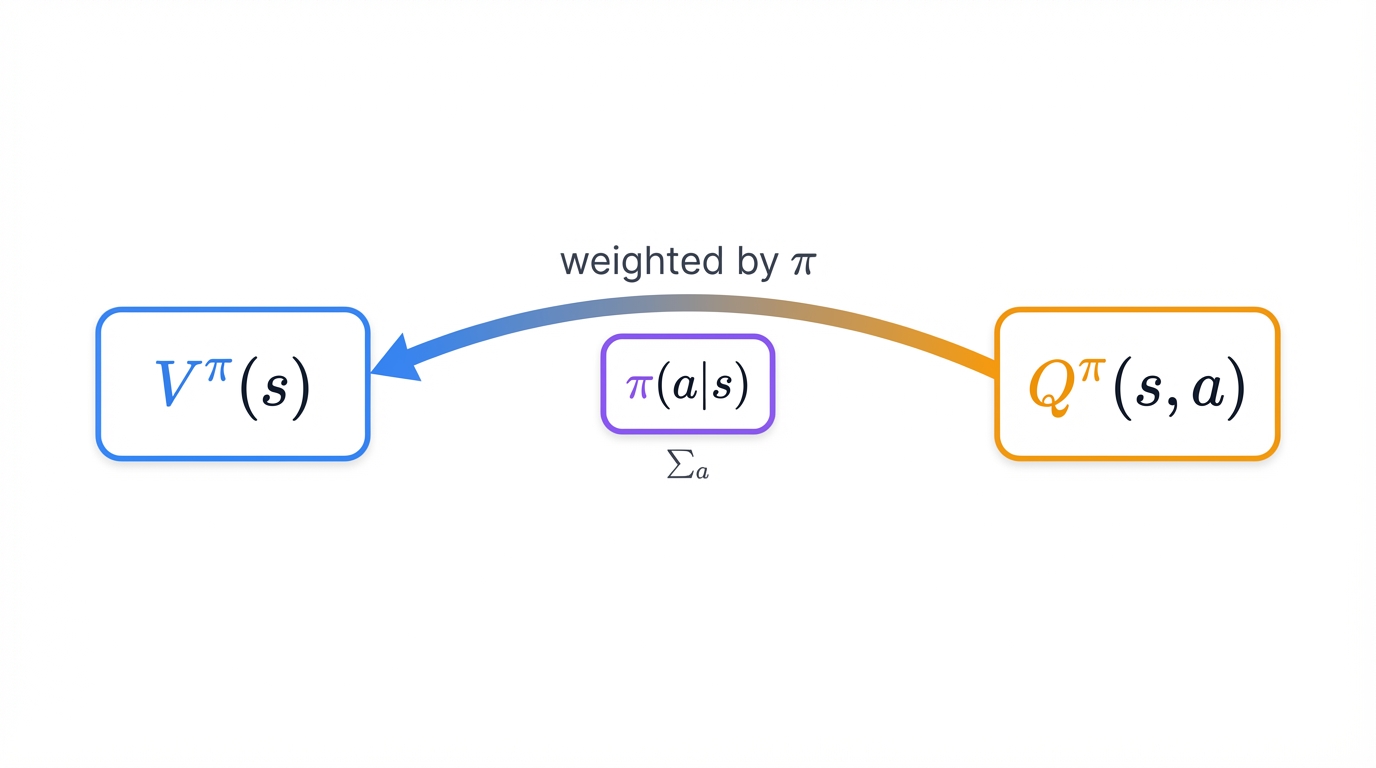
State Value Function V^π(s): Expected cumulative reward starting from state s and following policy π thereafter
V^π(s) = E[R_t + γR_{t+1} + γ²R_{t+2} + ... | S_t = s, π]
Action Value Function Q^π(s,a): Expected cumulative reward starting from state s, taking action a, then following policy π for all subsequent decisions
Q^π(s,a) = E[R_t + γR_{t+1} + γ²R_{t+2} + ... | S_t = s, A_t = a, π]
The relationship between these functions reveals the elegant structure of optimal decision-making, showing how state values emerge from action values weighted by policy probabilities, and how optimal policies select actions with maximum Q-values:
V^π(s) = Σ_a π(a|s) * Q^π(s,a)
Q-Learning: The Algorithm That Changed Everything
Q-Learning learns action values directly. No model required. This model-free approach revolutionized reinforcement learning by enabling agents to learn in completely unknown environments where the transition dynamics and reward function remain mysterious, opaque, and discoverable only through direct interaction with the world itself.
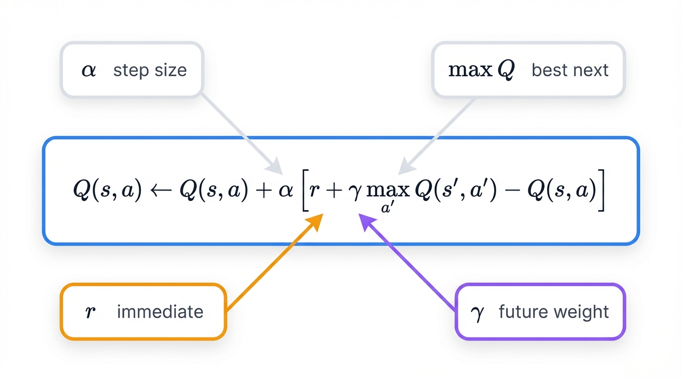
The Q-Learning Update Rule:
Q(s,a) ← Q(s,a) + α[r + γ max_a' Q(s',a') - Q(s,a)]
Breaking down the formula piece by piece:
- α: Learning rate (0 ≤ α ≤ 1) controlling how much new information affects the update—high values mean fast learning but potential instability
- r: Immediate reward received after taking action a in state s—the environment's instantaneous feedback
- γ: Discount factor determining the importance of future rewards relative to immediate payoffs—the agent's time preference
- max_a' Q(s',a'): Maximum Q-value for the next state across all possible actions—the best possible future value achievable
Key Parameters and Their Profound Effects:
Learning Rate (α): Set α=0.9 for rapid adaptation that risks instability and oscillation. Choose α=0.1 for stable, reliable convergence that progresses slowly. The tradeoff between speed and stability governs learning dynamics.
Discount Factor (γ): γ=0 creates myopic agents obsessed with immediate rewards, ignoring future consequences entirely. γ approaching 1.0 creates farsighted agents optimizing long-term outcomes, willing to sacrifice short-term gains for ultimate success. This single parameter shapes the agent's entire decision-making philosophy.
Exploration Rate (ε): The ε-greedy strategy balances exploration (trying new actions to discover better strategies) with exploitation (using known good actions to maximize immediate reward). Start with ε=1.0 for pure exploration, gradually decay to ε=0.01 for near-total exploitation as learning progresses.
Deep Reinforcement Learning: Scaling to Complex Worlds
Traditional tabular RL methods hit a wall. When state spaces explode—imagine every possible pixel configuration in an Atari game, every possible board position in Go, every possible sensor reading from an autonomous car—storing explicit Q-values for each state-action pair becomes computationally impossible, practically absurd, and theoretically hopeless.
Deep RL shatters this limitation. By combining neural networks with RL algorithms, we enable agents to handle high-dimensional inputs like images and continuous action spaces, learning compressed representations of value functions that generalize across similar states and scale to problems that seemed utterly intractable just a decade ago.
Deep Q-Networks (DQN): Neural Networks Meet Q-Learning
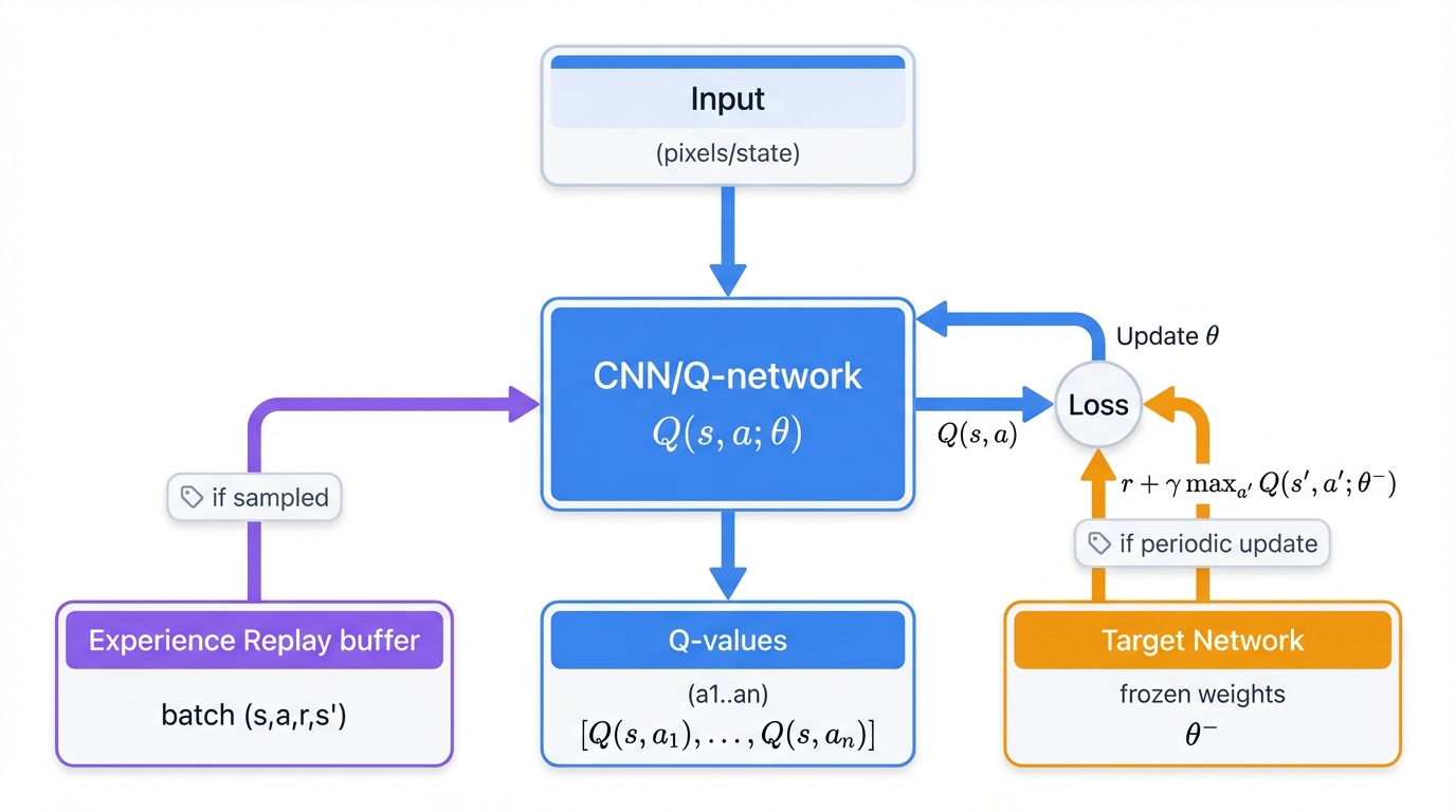
DQN replaces the Q-table with a neural network. Simple concept. Profound implications. This breakthrough enabled RL agents to master dozens of Atari games using only raw pixel inputs as observations, learning to play Space Invaders, Breakout, and Pong at superhuman levels without any hand-crafted features, without any domain-specific knowledge, with nothing but pixels, actions, and rewards.
Key Innovations That Made It Work:
- Experience Replay: Store experiences in a replay buffer, sample random batches for training, breaking the temporal correlations that destabilize neural network learning
- Target Network: Use a separate network for computing TD targets, update it periodically for stability, preventing the moving target problem that plagued earlier approaches
- CNN Architecture: Process high-dimensional visual inputs effectively through convolutional layers that learn hierarchical feature representations automatically
DQN Implementation Example
import torch
import torch.nn as nn
import torch.optim as optim
import numpy as np
from collections import deque
import random

class DQN(nn.Module):
    def __init__(self, state_size, action_size, hidden_size=64):
        super(DQN, self).__init__()
        self.network = nn.Sequential(
            nn.Linear(state_size, hidden_size),
            nn.ReLU(),
            nn.Linear(hidden_size, hidden_size),
            nn.ReLU(),
            nn.Linear(hidden_size, action_size)
        )

    def forward(self, x):
        return self.network(x)

class DQNAgent:
    def __init__(self, state_size, action_size, lr=0.001):
        self.state_size = state_size
        self.action_size = action_size
        self.memory = deque(maxlen=10000)
        self.epsilon = 1.0
        self.epsilon_decay = 0.995
        self.epsilon_min = 0.01

        # Neural networks
        self.q_network = DQN(state_size, action_size)
        self.target_network = DQN(state_size, action_size)
        self.optimizer = optim.Adam(self.q_network.parameters(), lr=lr)

        # Copy weights to target network
        self.update_target_network()

    def remember(self, state, action, reward, next_state, done):
        """Store experience in replay buffer"""
        self.memory.append((state, action, reward, next_state, done))

    def act(self, state):
        """Choose action using epsilon-greedy policy"""
        if random.random() <= self.epsilon:
            return random.choice(range(self.action_size))

        state_tensor = torch.FloatTensor(state).unsqueeze(0)
        q_values = self.q_network(state_tensor)
        return q_values.argmax().item()

    def replay(self, batch_size=32):
        """Train the network on a batch of experiences"""
        if len(self.memory) < batch_size:
            return

        batch = random.sample(self.memory, batch_size)
        states = torch.FloatTensor([e[0] for e in batch])
        actions = torch.LongTensor([e[1] for e in batch])
        rewards = torch.FloatTensor([e[2] for e in batch])
        next_states = torch.FloatTensor([e[3] for e in batch])
        dones = torch.BoolTensor([e[4] for e in batch])

        current_q_values = self.q_network(states).gather(1, actions.unsqueeze(1))
        next_q_values = self.target_network(next_states).max(1)[0].detach()
        target_q_values = rewards + (0.99 * next_q_values * ~dones)

        loss = nn.MSELoss()(current_q_values.squeeze(), target_q_values)

        self.optimizer.zero_grad()
        loss.backward()
        self.optimizer.step()

        # Decay epsilon
        if self.epsilon > self.epsilon_min:
            self.epsilon *= self.epsilon_decay

    def update_target_network(self):
        """Copy weights from main network to target network"""
        self.target_network.load_state_dict(self.q_network.state_dict())

# Training loop example
def train_dqn_agent(env, episodes=1000):
    agent = DQNAgent(state_size=4, action_size=2)  # Example sizes
    scores = []

    for episode in range(episodes):
        state = env.reset()
        total_reward = 0

        while True:
            action = agent.act(state)
            next_state, reward, done, _ = env.step(action)
            agent.remember(state, action, reward, next_state, done)

            state = next_state
            total_reward += reward

            if done:
                break

            # Train the agent
            if len(agent.memory) > 32:
                agent.replay()

        scores.append(total_reward)

        # Update target network every 100 episodes
        if episode % 100 == 0:
            agent.update_target_network()
            avg_score = np.mean(scores[-100:])
            print(f"Episode {episode}, Average Score: {avg_score:.2f}, Epsilon: {agent.epsilon:.3f}")

print("DQN implementation demonstrates how neural networks enable RL in complex environments")
This DQN implementation shows how neural networks replace Q-tables completely, enabling RL to tackle high-dimensional spaces that would choke tabular methods, handling continuous state representations with ease, and learning value function approximations that generalize beautifully across similar states through the magic of neural network function approximation.
Experience replay and target networks solve the stability problems that plagued every early attempt to combine deep learning with RL, providing the algorithmic foundations that transformed RL from academic curiosity into practical tool for solving real-world sequential decision problems.
Policy Gradient Methods: Direct Policy Optimization
Why learn value functions at all? Policy gradient methods take a radically different approach—they optimize the policy directly, using gradient ascent to climb the performance surface toward policies that maximize expected cumulative reward without ever explicitly representing action values.
This approach works particularly well for continuous action spaces where discretization becomes impractical, for stochastic policies where randomness is actually optimal, and for problems where smooth policy updates matter more than aggressive exploitation of learned value estimates.
Key Advantages That Drive Adoption:
- Handle continuous action spaces naturally without discretization artifacts or approximation errors
- Learn stochastic policies that are sometimes optimal, especially in partially observable environments
- Enjoy more stable convergence properties compared to value-based methods in many domains
- Better suited for cooperative multi-agent scenarios where coordination requires smooth policy updates
Popular Algorithms Dominating Modern RL:
- REINFORCE: Vanilla policy gradient with Monte Carlo returns—simple, elegant, high variance
- Actor-Critic: Combines policy gradients with value function estimation, using critics to reduce variance while maintaining policy gradient benefits
- PPO (Proximal Policy Optimization): Stable policy updates with clipped objectives that prevent destructively large policy changes, becoming the workhorse algorithm for many applications
- A3C (Asynchronous Actor-Critic): Parallel learning across multiple environments simultaneously, improving sample efficiency through diverse experience collection
Real-World Applications and Impact
Reinforcement learning escaped the laboratory. It solves real problems now, drives actual products, powers systems that millions of people interact with daily without realizing RL algorithms orchestrate their experiences, optimize their outcomes, and learn continuously from every interaction.
Game AI: Superhuman Performance Through Self-Play
AlphaGo and Beyond: March 2016. Seoul, South Korea. DeepMind's AlphaGo defeats world champion Lee Sedol in Go, a game with more possible positions than atoms in the observable universe, demonstrating that RL combined with deep learning could master domains previously thought to require uniquely human intuition, creativity, and strategic thinking.
AlphaZero generalized this success to chess and shogi using only self-play, learning from scratch without any human games, without opening books, without endgame databases, achieving superhuman performance through pure reinforcement learning combined with Monte Carlo tree search and deep neural networks.
OpenAI Five and Dota 2: Complex real-time strategy with imperfect information, team coordination, and combinatorial action spaces. OpenAI Five reached professional level through massive parallel training across thousands of CPUs and hundreds of GPUs, demonstrating that RL scales to extraordinarily complex multi-agent environments when given sufficient computational resources.
StarCraft II: AlphaStar mastered this incredibly complex RTS game, handling multi-tasking across dozens of units simultaneously, planning over multiple timescales from seconds to minutes, and executing real-time decisions at superhuman speed while maintaining strategic coherence that professional players found genuinely impressive and occasionally baffling.
Key Insights from Game AI Breakthroughs:
- Self-play discovers novel strategies unknown to human experts, sometimes revolutionizing competitive play
- Massive computational resources enable breakthrough performance—AlphaZero trained on 5,000 TPUs for hours
- Curriculum learning helps agents tackle complex tasks progressively, starting simple and gradually increasing difficulty
- Multi-agent training creates more robust policies that handle diverse opponents and unexpected strategies
Autonomous Systems: RL in the Physical World
Autonomous Driving: RL helps vehicles learn complex behaviors that resist traditional programming—lane changing in heavy traffic, merging onto highways at high speeds, navigating intersections with unpredictable pedestrians and cyclists. Simulation enables safe exploration of dangerous scenarios, while real-world fine-tuning handles the reality gap between simulation and actual driving conditions.
Robotics: Robot manipulation, walking gaits, and dexterous control benefit enormously from RL's trial-and-error approach. Teaching a robot hand to solve a Rubik's cube through RL demonstrates the power of this paradigm—the task involves complex contact dynamics, precise coordination, and planning over hundreds of moves, all learned through experience rather than explicit programming.
Drone Control: RL enables autonomous drone navigation through cluttered environments, obstacle avoidance at high speeds, and complex aerobatic maneuvers that exploit the full dynamics of quadrotor flight. The learned policies often discover control strategies that human pilots find counterintuitive but remarkably effective.
Industrial Applications Transforming Industries:
- Resource Management: Data center cooling optimization reduces energy consumption by 40%, traffic light coordination improves flow by 25%, power grid management balances supply and demand in real-time
- Financial Trading: Algorithmic trading strategies that adapt to changing market conditions, learning optimal execution policies that minimize market impact while achieving target positions
- Supply Chain: Inventory management under demand uncertainty, logistics optimization across complex distribution networks, demand forecasting that improves with every transaction
- Healthcare: Treatment protocol optimization that personalizes therapies to individual patients, drug dosing that balances efficacy against side effects, personalized medicine that learns optimal interventions from patient responses
Challenges and Future Directions
Important Consideration: While this approach offers significant benefits, it's crucial to understand its limitations and potential challenges as outlined in this section.
RL isn't magic. It faces real limitations. Understanding these challenges helps you choose appropriate techniques, set realistic expectations, and avoid painful failures when deploying RL in production systems where mistakes carry actual consequences.
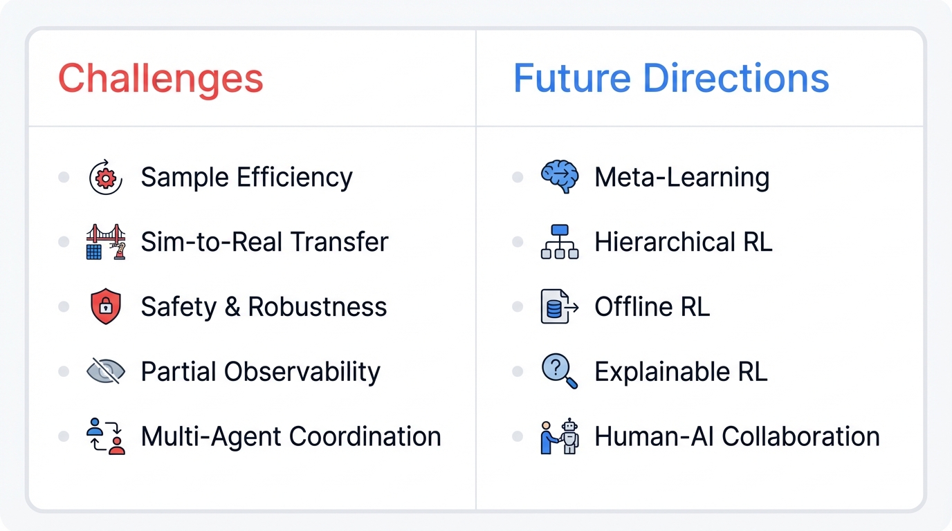
Current Challenges Blocking Wider Adoption:
- Sample Efficiency: RL algorithms often require millions of interactions to learn simple tasks—prohibitively expensive in real-world systems where data collection is slow, dangerous, or costly
- Sim-to-Real Transfer: Policies trained in perfect simulation often fail catastrophically in the real world due to modeling errors, unmodeled dynamics, and the reality gap that simulation can never fully close
- Safety and Robustness: Ensuring RL agents behave safely during both training and deployment remains unsolved—exploration can trigger dangerous actions, and learned policies may fail unpredictably on out-of-distribution states
- Partial Observability: Handling situations where the agent can't observe the full state requires memory, recurrence, or belief state tracking, significantly complicating learning
- Multi-Agent Coordination: Learning in environments with multiple interacting agents faces non-stationarity as other agents learn simultaneously, making convergence difficult and optimal policies elusive
Emerging Research Directions Shaping the Future:
- Meta-Learning: Learning to learn new tasks quickly from limited experience, enabling rapid adaptation to novel environments with minimal data
- Hierarchical RL: Learning at multiple time scales and abstraction levels, decomposing complex tasks into reusable subtasks that accelerate learning and improve generalization
- Offline RL: Learning from fixed datasets without environment interaction, enabling RL to leverage historical data and pre-collected experience safely
- Explainable RL: Understanding and interpreting agent decisions to build trust, enable debugging, and satisfy regulatory requirements in high-stakes applications
- Human-AI Collaboration: Agents that learn from and work with humans, combining the strengths of human intuition with machine learning's scalability and consistency
Getting Started with Reinforcement Learning
Ready to dive in? The RL ecosystem offers mature tools, comprehensive libraries, and standardized benchmarks that make getting started easier than ever before, though mastery still requires patience, experimentation, and many hours debugging why your agent is doing something utterly bizarre.
Essential Tools and Libraries:
- OpenAI Gym: Standard interface for RL environments providing hundreds of benchmarks from simple CartPole to complex Atari games
- Stable Baselines3: Reliable implementations of state-of-the-art RL algorithms with consistent APIs, thorough documentation, and proven performance
- Ray RLlib: Scalable RL library with distributed training support, enabling you to leverage multiple machines for parallel experience collection and training
- TensorFlow/PyTorch: Deep learning frameworks providing the neural network components that power modern deep RL algorithms
Learning Path from Beginner to Practitioner:
- Start with tabular methods like Q-learning in simple grid worlds to build intuition about the core concepts without neural network complexity
- Understand the exploration-exploitation trade-off thoroughly—this fundamental tension shapes all RL algorithm design
- Learn about function approximation and deep RL once you're comfortable with the basics and ready for high-dimensional problems
- Experiment with different algorithm families including value-based methods like DQN, policy-based approaches like REINFORCE, and actor-critic hybrids like PPO
- Tackle increasingly complex environments and real-world applications, gradually building the debugging skills and intuition that separate working implementations from perpetually broken experiments
Best Practices from Hard-Won Experience:
- Always start with the simplest approach that might work—sophisticated algorithms won't save poorly designed reward functions
- Use established benchmarks to validate your implementations before blaming the algorithm when your code doesn't work
- Pay careful attention to hyperparameter tuning because RL is notoriously sensitive to learning rates, batch sizes, and exploration schedules
- Implement proper logging and visualization for training progress since RL training curves are noisy and debugging requires detailed diagnostics
- Consider sample efficiency and computational costs in your choice of algorithms because that simple DQN might need 10 million samples and three days of GPU time