Part I: Understanding Sequential Processing
Section 1: Why Neural Networks Needed Memory
1.1 What Is Sequential Data?
Sequential Processing Power
RNNs revolutionized sequence modeling by maintaining memory across time steps. While transformers have gained prominence, RNN variants like LSTMs and GRUs remain valuable for specific sequential tasks.
Think about your data. Most of it has one critical feature: order matters. This is sequential data, and it's everywhere you look. Take language. "Dog bites man" paints one picture. "Man bites dog" tells a wildly different story. Same words. Different order. Completely different meaning.
Stock prices make sense only when you track their chronological flow. Audio signals? Pressure waves dancing through time. Videos? Image frames marching in precise sequence.
Here's what makes sequential data special: temporal dependency. What happens now depends on what happened before. You can't understand a story by reading random sentences. You can't grasp a conversation by hearing scrambled words. The order carries the meaning.
1.2 Why Traditional Neural Networks Failed at Sequences
The first successful neural networks had a simple design. Frank Rosenblatt's Perceptron started it all. Then came Feedforward Neural Networks—also called Multilayer Perceptrons. They work on one straightforward principle: information flows one direction, from input to output through hidden layers. No loops. No backward connections. Just clean, forward propagation.
This works brilliantly for static problems. Want to recognize what's in a photo? Perfect. But sequential data? That's where these networks hit a wall. The problem? They have no memory. None.
These networks treat every input as completely independent, as if nothing came before it. Feed a sentence to a feedforward network, and it analyzes each word in isolation, blind to the cumulative meaning built from their order. Why does this happen? Because feedforward networks are stateless systems.
Their output depends only on the current input and the learned weights. They carry no internal state influenced by past events. No history. No context. No memory. We needed something radically different for sequences—a shift from stateless pattern recognition to stateful, dynamic processing that could remember what it had seen.
1.3 Enter Recurrence: Giving Networks Memory
Recurrent Neural Networks (RNNs) made that shift. The key innovation? Internal memory, called the hidden state. How do they achieve this? Through a feedback loop—the output from a neuron at one time step feeds back into the network as part of the input for the next time step.
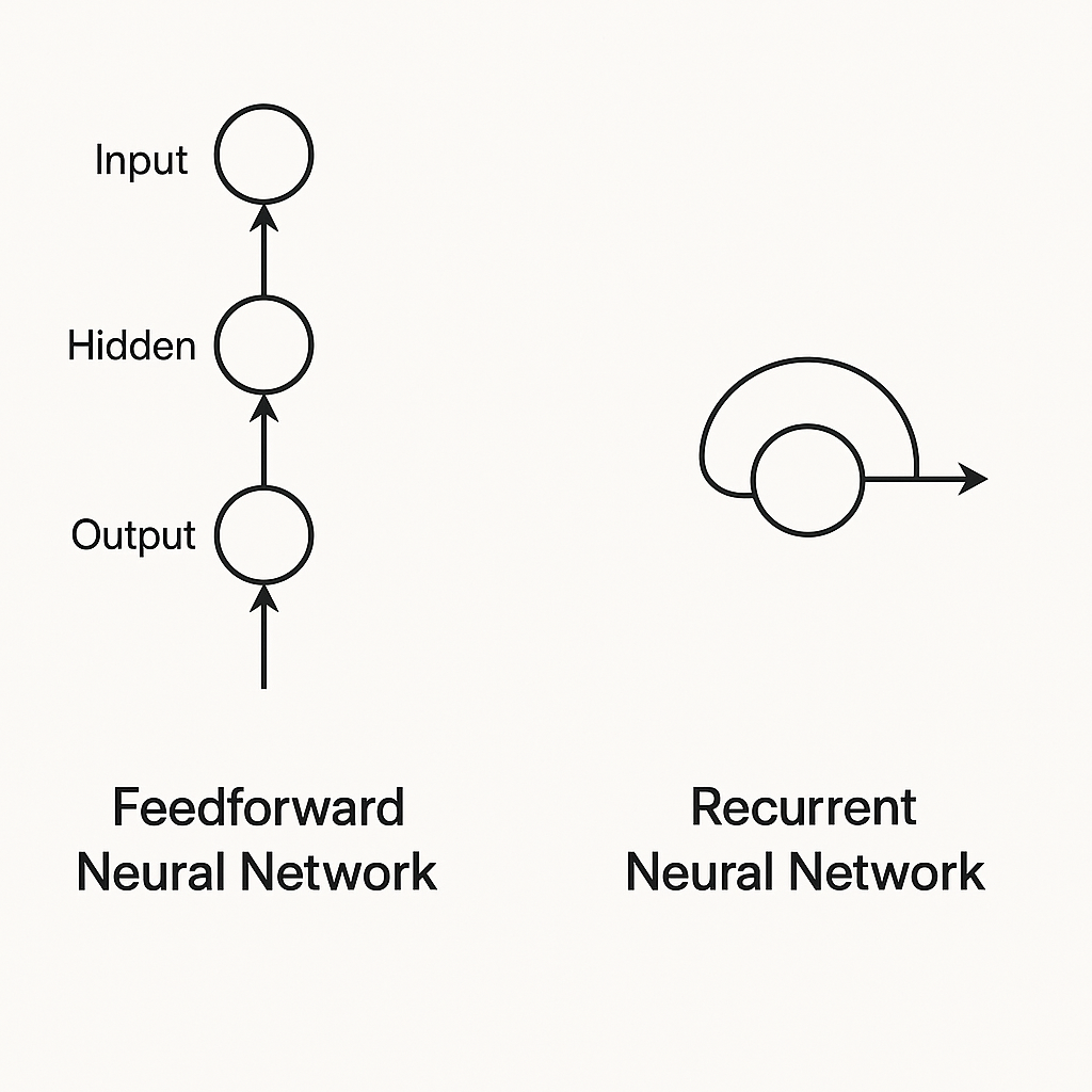
Comparison showing feedforward networks with linear data flow versus RNNs with feedback loops creating memory
This recurrent connection does something powerful: it allows the network to maintain a persistent state that works like a compressed summary of everything it has seen so far. At each step, the RNN updates its hidden state by combining new input with information from the previous state. Context builds. Understanding develops over time. The network remembers.
Comparison: Feedforward vs Recurrent Networks
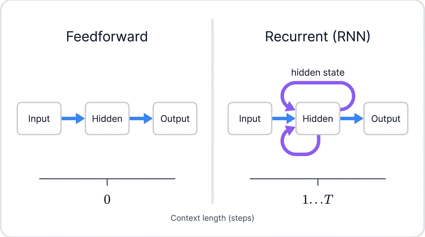
| Feature | Feedforward Neural Network | Recurrent Neural Network |
|---|---|---|
| Data Flow | One direction (input → output); no cycles | Cyclic; previous output feeds back as input |
| Memory | Stateless; no memory of past inputs | Stateful; maintains hidden state as memory |
| Input Handling | Requires fixed-size inputs; can't handle variable-length sequences | Can process variable-length sequences |
| Temporal Modeling | Can't capture time-based patterns | Designed specifically for temporal dependencies |
| Example Uses | Image classification, object detection, tabular data | Natural language processing, speech recognition, time-series forecasting |
Section 2: How RNNs Came to Be: A Historical Journey
The story of RNNs isn't a straight line. It's multiple streams of research—neuroscience, statistics, mathematics—converging over decades, punctuated by algorithmic breakthroughs that transformed theory into working reality.
2.1 Early Brain Inspiration (1900s-1940s)
The concept of recurrence in the brain predates computers by decades. In the early 1900s, Santiago Ramón y Cajal discovered structures he called "recurrent semicircles" in brain tissue. Rafael Lorente de Nó identified "recurrent, reciprocal connections" and speculated these loops might unlock the secret to complex neural behaviors.
By the 1940s, our understanding evolved. Scientists started seeing the brain as a system built on feedback loops rather than one-way information flow. Donald Hebb proposed "reverberating circuits" as a mechanism for short-term memory. Then, in 1943, Warren McCulloch and Walter Pitts published their groundbreaking paper.
They modeled neurons mathematically. They explored networks with cycles. They proposed that past events could influence ongoing neural activity. The seeds were planted.
2.2 The Computer Age Begins: Perceptrons and Early Models (1950s-1970s)
Neural networks entered the spotlight in 1958. Frank Rosenblatt invented the Perceptron—a simple, single-layer network capable of pattern recognition. Revolutionary for its time. But in 1969, Marvin Minsky and Seymour Papert published Perceptrons, highlighting critical limitations like the inability to solve the XOR problem.
Funding dried up. Enthusiasm waned. The first "AI winter" descended—a period of reduced interest and investment in artificial intelligence research. Yet the idea of recurrence persisted.
Rosenblatt himself had described "closed-loop cross-coupled" perceptrons with recurrent connections back in the 1960s. The missing piece? A reliable training method for complex networks. Over the following years, researchers like Seppo Linnainmaa and Paul Werbos developed the mathematics behind backpropagation—an algorithm that would eventually revolutionize how neural networks learn.
2.3 The Comeback and Modern RNNs (1980s-1990s)
The 1980s brought resurgence. A major turning point arrived in 1982 with John Hopfield's paper introducing Hopfield Networks. These networks bridged recurrent architectures with ideas from statistical mechanics, like the Ising model of magnetism. Scientists saw them as "attractor networks" capable of storing and retrieving memories. The foundation was set.
Then came 1986. David Rumelhart, Geoffrey Hinton, and Ronald Williams published their landmark paper, thrusting backpropagation into the spotlight and formally introducing what we now call modern recurrent neural networks. Soon after, influential models emerged: the Jordan network in 1986, the Elman network in 1990, both applying RNNs to cognitive science.
Key Milestones in RNN Development
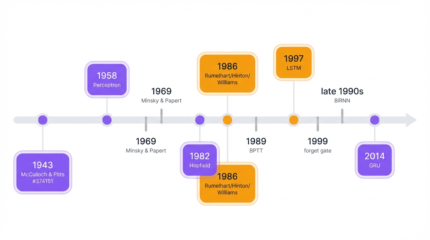
Training recurrent networks required a new approach to backpropagation. This led to Backpropagation Through Time (BPTT), developed by Ronald Williams and David Zipser in 1989. BPTT worked by 'unrolling' the network across time steps to compute gradients over long sequences. Clever. Powerful. But it revealed a major challenge.
The vanishing gradient problem. Researchers like Sepp Hochreiter in 1991 and Yoshua Bengio and colleagues in 1994 analyzed how error signals diminish as they propagate backward through lengthy sequences. The signals fade. Learning becomes increasingly difficult. The problem demanded a solution.
2.4 The Gated Revolution: LSTM and Beyond (1997-Present)
In 1997, Sepp Hochreiter and Jürgen Schmidhuber directly confronted the vanishing gradient challenge. They invented Long Short-Term Memory (LSTM) networks. LSTMs introduced special memory components and gates controlling information flow, designed specifically to maintain signals over long sequences. In 1999, Felix Gers and colleagues added the "forget gate," making these models even more powerful.
The late 1990s brought another innovation: Bidirectional RNNs by Mike Schuster and Kuldip Paliwal. These networks process data both forwards and backwards, understanding context from past and future simultaneously. Then, in 2014, Kyunghyun Cho and his team introduced the Gated Recurrent Unit (GRU)—a simplified LSTM variant that matches its performance but runs more efficiently.
Key Milestones in RNN History
| Date | Milestone | Key People | Why It Mattered |
|---|---|---|---|
| 1943 | McCulloch-Pitts Neuron | Warren McCulloch & Walter Pitts | First mathematical model of a neuron; considered networks with cycles |
| 1949 | Hebbian Learning | Donald Hebb | Proposed "cells that fire together, wire together" - foundational learning principle |
| 1958 | The Perceptron | Frank Rosenblatt | First trainable neural network, groundwork for modern machine learning |
| 1974 | Backpropagation (early) | Paul Werbos | Core algorithm for training multilayer networks (popularized later) |
| 1982 | Hopfield Network | John Hopfield | RNN that functions as associative memory, linked neural networks to statistical mechanics |
| 1986 | Modern RNN Concept | Rumelhart, Hinton, Williams | Formalized modern RNN architecture and popularized backpropagation |
| 1989 | Backpropagation Through Time | Williams & Zipser | Standard algorithm for training RNNs by unrolling through time |
| 1991-94 | Vanishing Gradient Problem | Hochreiter; Benigo et al. | Identified the major barrier preventing RNNs from learning long sequences |
| 1997 | LSTM Networks | Hochreiter & Schmidhuber | Solved vanishing gradients with gated memory cells |
| 2014 | GRU Networks | Cho et al. | Simplified gated architecture, often as good as LSTM but more efficient |
Section 3: How RNNs Actually Work
3.1 The Basic RNN Architecture
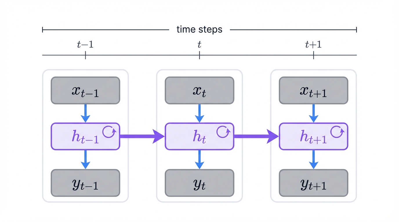
At its core, an RNN is surprisingly simple. It's a feedforward network with one key addition: a feedback loop. At each time step, the network takes two inputs—the current data point and its own previous hidden state. It produces two outputs: a prediction and a new hidden state. That's it.
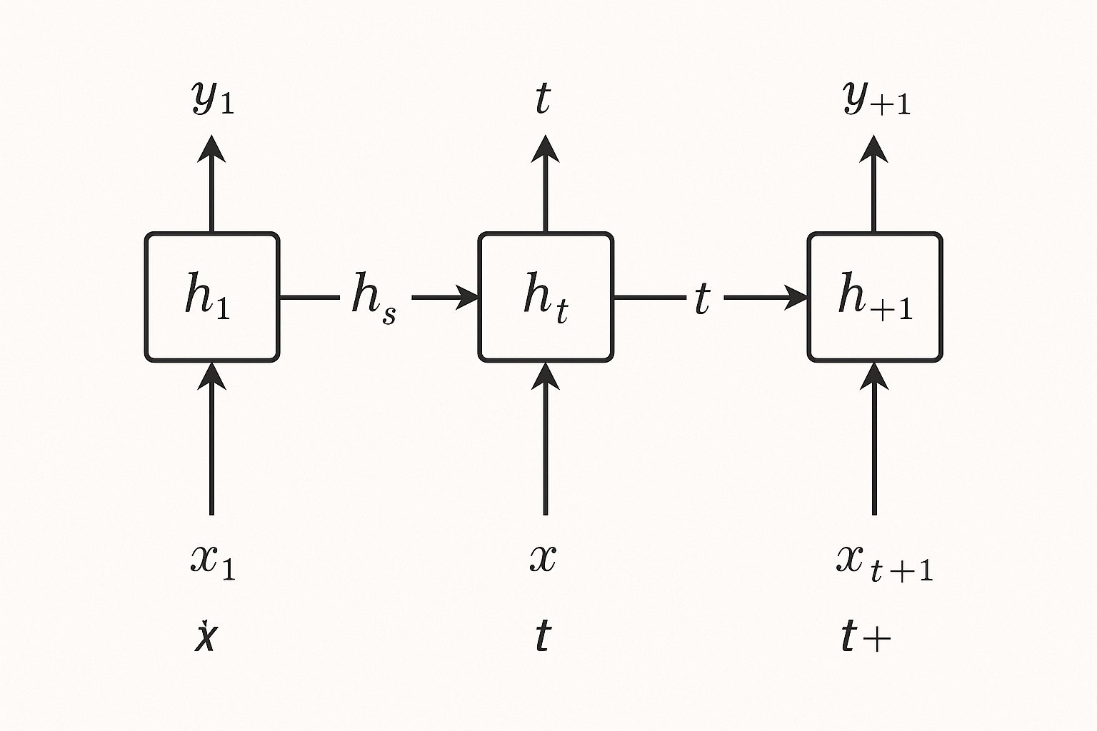
Step-by-step visualization of how information flows through an RNN with memory states
Section 4: Advanced RNN Architectures
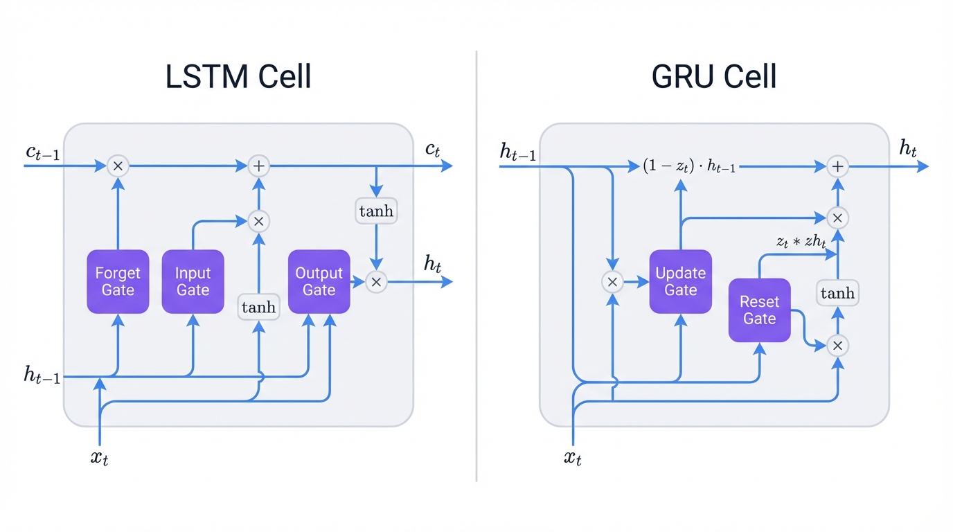
4.1 Long Short-Term Memory (LSTM)
LSTMs solve the vanishing gradient problem through sophisticated gating. They use three gates—forget, input, and output—to control information flow and maintain long-term dependencies. Each gate decides what information to keep, what to discard, and what to output, creating a network that can remember important patterns across hundreds or thousands of time steps.
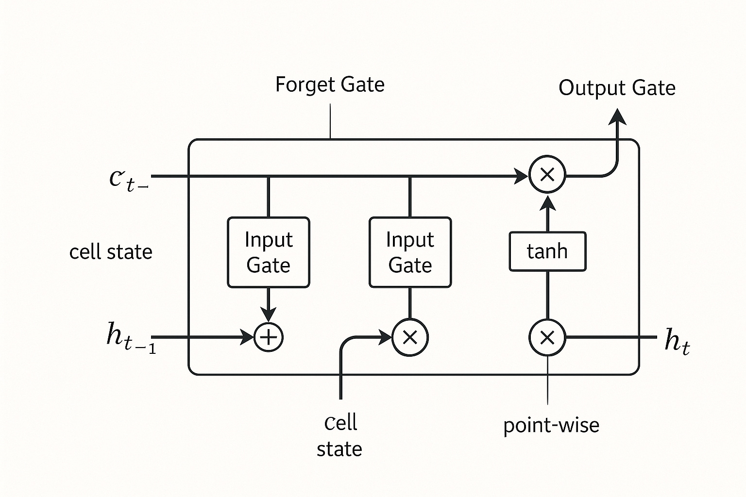
LSTM cell architecture showing gates and information flow
4.2 Gated Recurrent Units (GRU)
GRUs simplify LSTM architecture. They combine the forget and input gates into a single update gate, making them computationally more efficient while maintaining similar performance. Fewer parameters. Faster training. Same power. For many applications, GRUs deliver LSTM-level results with less computational overhead.
Section 5: RNNs in Action: Real-World Applications
5.1 Natural Language Processing
RNNs revolutionized NLP. They finally gave machines the ability to understand context in language. Real context. Not just isolated words.
- Language Modeling: Predicting the next word in a sequence. This forms the foundation for text generation systems that can write coherent paragraphs, complete your sentences, and generate human-like text.
- Machine Translation: Sequence-to-sequence models use an encoder RNN to read the source language and a decoder RNN to generate the translation, capturing nuance and context that word-for-word translation misses.
- Sentiment Analysis: Analyzing emotional tone in text by processing word sequences and building contextual understanding of negation, sarcasm, and subtle emotional cues that single-word analysis would miss.
- Named Entity Recognition: Identifying people, places, and organizations in text, which demands contextual understanding—is "Washington" a person or a place? The surrounding context tells the story.
5.2 Speech Recognition
- Acoustic Modeling: Mapping acoustic features from audio signals to phonemes—the basic speech sounds that form words. RNNs capture the temporal dynamics of how sounds flow and blend together.
- End-to-End Speech Recognition: Directly mapping audio to text, achieving impressive accuracy by learning the entire transformation from sound waves to written words in a single, integrated model.
5.3 Time Series Analysis
- Financial Forecasting: Modeling stock prices, currency rates, and economic indicators by learning complex temporal patterns and dependencies in historical market data.
- Weather Prediction: Learning intricate temporal dynamics from historical weather data, capturing how atmospheric conditions evolve and interact over time to predict future states.
- Demand Forecasting: Predicting product demand based on historical sales patterns, seasonal trends, and cyclical behaviors that emerge when you analyze data across time.
5.4 Computer Vision Applications
- Video Analysis: Action recognition, video captioning, and temporal modeling in sequences of frames, understanding how visual scenes evolve and change over time.
- Image Captioning: Combining CNNs for image understanding with RNNs for language generation to describe images in natural language, bridging vision and text in a single integrated system.
- Handwriting Recognition: Understanding stroke sequences over time, capturing the temporal dynamics of how humans write to recognize characters and words from pen movements.
Section 6: Challenges and Limitations
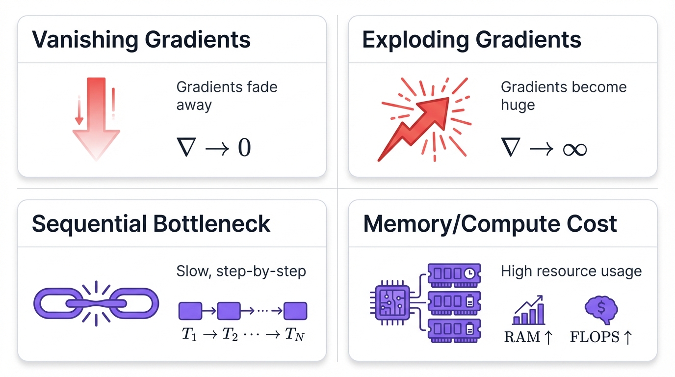
6.1 The Vanishing Gradient Problem
Even with LSTMs and GRUs, this remains a challenge. A persistent one.
- What happens: Gradients become exponentially smaller as they propagate back through time. Each layer diminishes the signal a little more until it effectively disappears.
- Why it matters: The network can't learn long-term dependencies. It forgets. Information from early time steps vanishes before it can influence learning.
- Solutions: Gated architectures like LSTM and GRU help significantly. Gradient clipping prevents explosive growth. Careful initialization sets networks up for success from the start.
6.2 Sequential Processing Bottleneck
RNNs process sequences step by step. One after another. This creates fundamental constraints.
- Slow training: You can't parallelize processing within a single sequence. Each step depends on the previous one, forcing sequential computation that modern GPUs can't accelerate the way they can with other architectures.
- Inference latency: Networks must generate tokens one at a time, waiting for each output before computing the next, creating delays in real-time applications.
- Scalability issues: Processing very long sequences becomes prohibitively slow and resource-intensive, limiting the practical length of sequences you can handle.
This limitation drove the development of Transformers, which solve the parallelization problem through attention mechanisms that allow simultaneous processing of entire sequences.
6.3 Memory and Computational Requirements
- Memory usage: You must store hidden states for the entire sequence during training. Long sequences demand substantial memory, limiting batch sizes and sequence lengths you can practically handle.
- Computational cost: RNNs often have more parameters than comparable feedforward networks, requiring more operations per forward pass and increasing training time and resource requirements.
- Training time: The sequential nature makes training inherently slower. You can't take full advantage of parallel processing hardware, extending the time needed to train models on large datasets.
6.4 Instability and Training Difficulties
- Exploding gradients: Gradients can grow exponentially large—the opposite of vanishing—causing numerical instability, failed training runs, and NaN values that destroy learning progress.
- Sensitivity to initialization: Poor initialization can prevent the network from learning at all. You need careful weight initialization strategies to give the network a fighting chance at convergence.
- Hyperparameter tuning: Learning rates, hidden state sizes, and architectural choices require careful tuning. Small changes can mean the difference between successful learning and complete failure.
Section 7: Modern Context and Legacy
7.1 The Rise of Transformers
The 2017 paper "Attention Is All You Need" introduced Transformers. They brought several advantages over RNNs that transformed the field:
- Parallelization: They can process entire sequences simultaneously, taking full advantage of modern GPU architectures to dramatically accelerate training and inference.
- Long-range dependencies: Self-attention provides direct connections between all positions in a sequence, eliminating the distance problem that plagues RNNs trying to remember early information.
- Scalability: You can train them efficiently on massive datasets with billions of parameters, unlocking performance levels that RNNs couldn't reach due to their sequential constraints.
This ushered in the current era of large language models like GPT and BERT, which dominate modern NLP applications and continue pushing the boundaries of what's possible with sequence modeling.
7.2 Where RNNs Still Matter
Despite Transformers' success, RNNs remain important in specific domains where their characteristics provide real advantages:
- Streaming applications: Perfect for processing data as it arrives in real-time. RNNs naturally handle streaming inputs without needing to buffer entire sequences before making predictions.
- Resource constraints: More efficient for smaller models and edge devices where memory and computation are limited. A well-designed RNN can deliver strong performance with fewer parameters than comparable Transformer models.
- Specific domains: Some tasks still benefit from the inductive biases of RNNs—their built-in assumptions about sequential structure that can accelerate learning when those assumptions match the problem.
- Real-time processing: Lower latency for certain sequential decision-making tasks where you need immediate responses based on streaming input without waiting to accumulate context.
7.3 Lessons Learned
RNNs taught the field crucial lessons about sequence modeling that extend far beyond their specific architecture:
- Memory matters: Stateful models are essential for sequential data. You can't understand sequences without maintaining context across time. This insight drives all modern sequence models.
- Architecture design: Gating mechanisms are powerful tools for controlling information flow and solving gradient problems. The gates in LSTMs and GRUs pioneered techniques now used throughout deep learning.
- Inductive biases: Built-in assumptions about data structure—like sequentiality—help learning by constraining the hypothesis space and focusing the model on relevant patterns.
- Trade-offs exist: You must balance expressiveness, efficiency, and trainability. More powerful models aren't always better if they're too slow to train or too resource-intensive to deploy.
Conclusion: RNNs' Lasting Impact
Recurrent Neural Networks mark a turning point in AI. They were among the first to give machines memory—the ability to remember and understand sequences. This capability paved the way for countless modern AI applications. While cutting-edge models like Transformers dominate current research, RNNs laid foundational principles of sequential thinking that still influence AI today.
Look back at the journey. Simple perceptrons evolved into complex RNNs through decades of innovation. Solving persistent problems sparked breakthroughs. The vanishing gradient issue led to LSTMs and GRUs. The need for efficient sequence processing drove the creation of Transformers. Each new idea built on previous insights while overcoming specific limitations.
Today, RNNs remain valuable where their characteristics—processing one piece at a time, remembering important information, working with streaming data—offer real advantages. They're an important part of the AI toolkit. Anyone serious about AI should understand them.
The story of RNNs teaches us something important: progress comes from tackling fundamental problems with clever designs. As we look to the future, the lessons from RNNs—about memory, gradients, and matching architecture to data—continue inspiring researchers finding solutions for tomorrow's challenges. The beat goes on. The music plays. And neural networks keep learning, one sequence at a time.
