1. Why High-Dimensional Data Breaks Everything
High-dimensional data destroys clustering algorithms. Watch it happen. The "Curse of Dimensionality" spreads your data thin, scatters points across vast empty spaces, and turns distance calculations into computational nightmares. Your clustering algorithms depend on measuring nearness and farness, but in high dimensions, that distinction evaporates like morning mist.
Key Concept: Master this foundation first—everything that follows builds on understanding how dimensionality breaks traditional distance-based algorithms.
PCA rescues you. It finds the most important directions in your data, the patterns that actually matter, and throws away the noise. Instead of wrestling with hundreds of features that confuse your algorithms, you work with a handful of principal components that capture the essential structure. This transformation makes clustering not just possible—it makes it effective.
1.1 The Curse of Dimensionality: Why More Features Make Things Worse
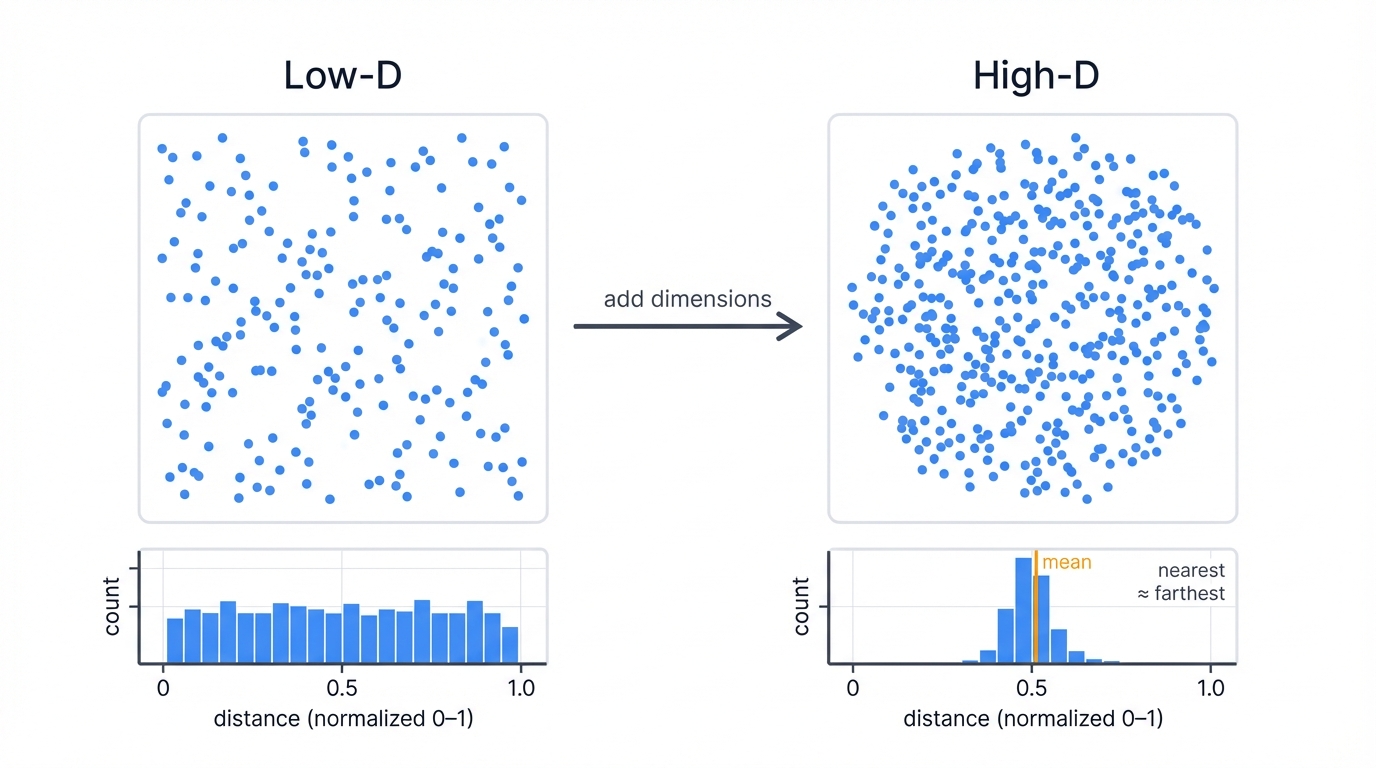
More features create bigger problems. Each new dimension expands your space exponentially, spreading data points farther and farther apart, creating a universe of emptiness where your algorithms suffocate. In low dimensions, neighborhoods have meaning—points cluster together, separated by clear distances. But add dimensions? Everything changes. Your nearest neighbor and farthest neighbor converge to roughly the same distance, and the entire concept of "close" versus "far" collapses into mathematical rubble.
Three disasters strike simultaneously when you work with high-dimensional data. Computational explosion hits first—your distance calculations require exponentially more processing power and memory with each added dimension, transforming quick operations into glacial crawls that can take hours or days to complete on real datasets. Then overfitting paradise emerges—your models discover phantom patterns in the noise, fitting to random fluctuations rather than genuine signal, creating relationships that evaporate when tested on new data. Finally, visualization impossibility blinds you completely—humans can perceive three dimensions, maybe fake a fourth with color, but beyond that we're working blind, unable to see the patterns we're trying to find or validate the clusters we think we've discovered.
You need dimensionality reduction that strips away the noise while keeping the signal, that compresses hundreds of dimensions into a handful of meaningful coordinates, and that does this automatically without requiring you to manually select which features matter and which don't.
1.2 Seeing the Curse in Action: A Demonstration
Want proof? Let's watch high dimensions destroy distance-based algorithms in real time:
import numpy as np
import matplotlib.pyplot as plt
from scipy.spatial.distance import pdist, squareform
from sklearn.neighbors import NearestNeighbors

# Demonstrate curse of dimensionality with synthetic data
np.random.seed(42)

print("Curse of Dimensionality Demonstration")
print("=" * 37)

# Test across different dimensions
dimensions = [2, 5, 10, 20, 50, 100]
n_samples = 1000

results = []

for d in dimensions:
    # Generate random data in d dimensions
    X = np.random.normal(0, 1, (n_samples, d))

    # Calculate all pairwise distances
    distances = pdist(X, metric='euclidean')

    # Find nearest and farthest distances from first point
    nn = NearestNeighbors(n_neighbors=2)  # 2 because first neighbor is the point itself
    nn.fit(X)
    nearest_distances, _ = nn.kneighbors(X[:1])
    nearest_dist = nearest_distances[0][1]  # Distance to nearest neighbor
    farthest_dist = np.max(distances)

    # Calculate statistics
    mean_dist = np.mean(distances)
    std_dist = np.std(distances)
    nearest_to_farthest_ratio = nearest_dist / farthest_dist

    results.append({
        'dimensions': d,
        'mean_distance': mean_dist,
        'std_distance': std_dist,
        'nearest_distance': nearest_dist,
        'farthest_distance': farthest_dist,
        'ratio': nearest_to_farthest_ratio
    })

    print(f"\nDimensions: {d}")
    print(f"  Mean distance: {mean_dist:.3f}")
    print(f"  Std distance: {std_dist:.3f}")
    print(f"  Nearest neighbor distance: {nearest_dist:.3f}")
    print(f"  Farthest distance: {farthest_dist:.3f}")
    print(f"  Nearest/Farthest ratio: {nearest_to_farthest_ratio:.3f}")
    print(f"  Coefficient of variation: {std_dist/mean_dist:.3f}")

# Demonstrate concentration of distances
print(f"\nKey Insight: Distance Concentration")
print("-" * 32)
print("As dimensions increase:")
print("- All distances become similar (low coefficient of variation)")
print("- Nearest and farthest distances converge (ratio approaches 1)")
print("- Notion of 'close' vs 'far' loses meaning")

# Visualize the effect
fig, (ax1, ax2) = plt.subplots(1, 2, figsize=(12, 5))

# Plot 1: Distance concentration
dims = [r['dimensions'] for r in results]
coeffs = [r['std_distance']/r['mean_distance'] for r in results]
ax1.plot(dims, coeffs, 'bo-')
ax1.set_xlabel('Dimensions')
ax1.set_ylabel('Coefficient of Variation')
ax1.set_title('Distance Concentration Effect')
ax1.grid(True)

# Plot 2: Nearest/Farthest ratio
ratios = [r['ratio'] for r in results]
ax2.plot(dims, ratios, 'ro-')
ax2.set_xlabel('Dimensions')
ax2.set_ylabel('Nearest/Farthest Distance Ratio')
ax2.set_title('Loss of Distance Discrimination')
ax2.grid(True)

plt.tight_layout()
plt.show()

print(f"\nConclusion: High-dimensional spaces make clustering nearly impossible!")
print("PCA rescues us by finding lower-dimensional representations that preserve structure.")
This code exposes the curse with brutal clarity. Watch what happens as you add dimensions—distances cluster around their mean like moths around a flame, the coefficient of variation plummets, and the ratio between nearest and farthest neighbors creeps toward 1. Your clustering algorithm loses its ability to distinguish between truly similar points and random noise, rendering k-means, hierarchical clustering, and DBSCAN nearly useless in their raw form.
1.3 PCA as the Solution: Finding What Matters
PCA cuts through the noise. It identifies the directions where your data actually varies, where the signal lives, and ignores the dimensions where you just have random fluctuations bouncing around the mean. These directions—your principal components—become your new features, your new coordinate system, the lens through which you view your data transformed into something you can actually work with.
Think of it like this: your thousand-dimensional dataset is casting shadows on lower-dimensional walls, and PCA finds the angle that produces the most informative shadow. You might discover that 95% of your data's variation lives in just 10 or 50 dimensions, which means you can discard hundreds of noisy features without losing the patterns that make your data unique. This compression makes visualization possible, clustering tractable, and analysis meaningful again.
The insight that powers PCA? Most high-dimensional datasets have hidden structure. Features correlate with each other, creating redundancy. Random noise lives in its own little corner. The true signal concentrates in a lower-dimensional subspace, and PCA discovers that subspace automatically, requiring only that you specify how much variance you want to preserve.
2. The Mathematical Foundation: Eigenvectors and Variance
PCA relies on linear algebra's most powerful tools. It finds directions—eigenvectors—where your data spreads out the most, then uses those directions to build a new coordinate system that captures maximum information with minimum dimensions.
2.1 The Covariance Matrix: Measuring Relationships
Everything begins with the covariance matrix. Your data matrix X contains n samples and p features. Center it by subtracting the mean from each feature, then compute the covariance matrix C:
$$C = \frac{1}{n-1}X^TX$$
This symmetric matrix holds the key to understanding your data's structure. Each entry C[i,j] quantifies how features i and j vary together, revealing the correlation structure that PCA will exploit:
- Positive values signal features that rise and fall together, creating redundancy you can compress
- Negative values reveal inverse relationships where one feature increases as the other decreases
- Zero means independence—the features vary without any linear relationship between them
- Diagonal entries contain each feature's variance, the spread you'll try to preserve in fewer dimensions
2.2 Eigendecomposition: Finding Principal Directions
Now comes the magic. Decompose the covariance matrix into its fundamental building blocks:
$$C = VDV^T$$
This factorization reveals everything:
- V contains eigenvectors as columns—each one defines a principal component direction
- D holds eigenvalues on the diagonal—these measure variance along each component
Each eigenvector points in a direction through your feature space. The corresponding eigenvalue tells you how much your data varies along that direction. Large eigenvalues mark important directions where data spreads out. Small eigenvalues indicate directions with minimal variation—mostly noise you can safely discard.
2.3 The Transformation Process
Six steps transform high-dimensional chaos into manageable structure:
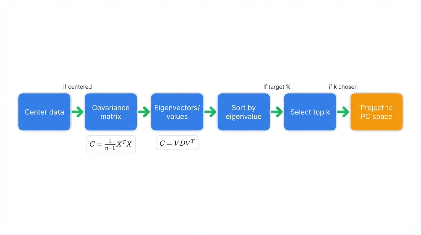
- Center the data: Subtract each feature's mean, moving the origin to your data's center point
- Compute covariance matrix: Calculate how every pair of features varies together
- Find eigenvalues and eigenvectors: Extract the principal directions from the covariance structure
- Sort by eigenvalue: Order components from most important to least important
- Select top k components: Decide how many dimensions you need to preserve target variance
- Transform data: Project your samples onto the new coordinate system defined by principal components
Working Example: Complete PCA Implementation
import numpy as np
import matplotlib.pyplot as plt
from sklearn.datasets import make_blobs
from sklearn.preprocessing import StandardScaler

class PCAFromScratch:
    """
    Principal Component Analysis implementation from scratch
    to demonstrate the mathematical concepts step by step.
    """

    def __init__(self, n_components=None):
        self.n_components = n_components
        self.components_ = None
        self.explained_variance_ = None
        self.explained_variance_ratio_ = None
        self.mean_ = None

    def fit(self, X):
        """
        Fit PCA on the data matrix X.

        Parameters:
        X: array-like, shape (n_samples, n_features)
        """
        print("PCA Step-by-Step Implementation")
        print("=" * 35)

        # Step 1: Center the data
        print("Step 1: Centering the data")
        self.mean_ = np.mean(X, axis=0)
        X_centered = X - self.mean_

        print(f"  Original data shape: {X.shape}")
        print(f"  Data mean: {self.mean_[:3]}..." if len(self.mean_) > 3 else f"  Data mean: {self.mean_}")
        print(f"  Centered data mean: {np.mean(X_centered, axis=0)[:3]}..." if X_centered.shape[1] > 3 else f"  Centered data mean: {np.mean(X_centered, axis=0)}")

        # Step 2: Compute covariance matrix
        print("\nStep 2: Computing covariance matrix")
        n_samples = X.shape[0]
        cov_matrix = (X_centered.T @ X_centered) / (n_samples - 1)

        print(f"  Covariance matrix shape: {cov_matrix.shape}")
        print(f"  Sample covariance values:")
        for i in range(min(3, cov_matrix.shape[0])):
            for j in range(min(3, cov_matrix.shape[1])):
                print(f"    Cov[{i},{j}] = {cov_matrix[i,j]:.4f}")

        # Step 3: Eigendecomposition
        print("\nStep 3: Eigenvalue decomposition")
        eigenvalues, eigenvectors = np.linalg.eigh(cov_matrix)

        # Sort by eigenvalues (descending)
        idx = eigenvalues.argsort()[::-1]
        eigenvalues = eigenvalues[idx]
        eigenvectors = eigenvectors[:, idx]

        print(f"  Number of eigenvalues: {len(eigenvalues)}")
        print(f"  Top 5 eigenvalues: {eigenvalues[:5]}")

        # Step 4: Select components
        if self.n_components is None:
            self.n_components = len(eigenvalues)

        print(f"\nStep 4: Selecting top {self.n_components} components")
        self.components_ = eigenvectors[:, :self.n_components].T
        self.explained_variance_ = eigenvalues[:self.n_components]

        # Calculate explained variance ratio
        total_variance = np.sum(eigenvalues)
        self.explained_variance_ratio_ = self.explained_variance_ / total_variance
        cumulative_variance = np.cumsum(self.explained_variance_ratio_)

        print(f"  Individual explained variance ratios:")
        for i, ratio in enumerate(self.explained_variance_ratio_[:5]):
            print(f"    PC{i+1}: {ratio:.4f} ({ratio*100:.1f}%)")

        print(f"  Cumulative explained variance:")
        for i, cum_ratio in enumerate(cumulative_variance[:5]):
            print(f"    PC1-{i+1}: {cum_ratio:.4f} ({cum_ratio*100:.1f}%)")

        return self

    def transform(self, X):
        """Transform data to principal component space."""
        print(f"\nStep 5: Transforming data to PC space")
        X_centered = X - self.mean_
        X_transformed = X_centered @ self.components_.T

        print(f"  Original data shape: {X.shape}")
        print(f"  Transformed data shape: {X_transformed.shape}")
        print(f"  Dimensionality reduction: {X.shape[1]} → {X_transformed.shape[1]} features")

        return X_transformed

    def fit_transform(self, X):
        """Fit PCA and transform data in one step."""
        return self.fit(X).transform(X)

    def inverse_transform(self, X_transformed):
        """Transform data back to original space (approximate)."""
        X_reconstructed = X_transformed @ self.components_ + self.mean_
        return X_reconstructed

# Demonstration
print("COMPREHENSIVE PCA DEMONSTRATION")
print("=" * 35)

# Generate synthetic high-dimensional data with known structure
np.random.seed(42)
n_samples = 200
n_features = 10

# Create data with intrinsic 2D structure embedded in 10D space
true_2d = np.random.randn(n_samples, 2)
# Embed in higher dimensions with noise
embedding_matrix = np.random.randn(2, n_features)
X_high_dim = true_2d @ embedding_matrix + 0.1 * np.random.randn(n_samples, n_features)

print(f"Generated data: {n_samples} samples, {n_features} features")
print(f"True underlying dimensionality: 2")

# Apply our PCA implementation
pca = PCAFromScratch(n_components=5)
X_pca = pca.fit_transform(X_high_dim)

# Analysis of results
print(f"\n" + "="*50)
print("RESULTS ANALYSIS")
print("="*50)

print(f"Dimensionality reduction achieved:")
print(f"  Original: {X_high_dim.shape[1]} dimensions")
print(f"  Reduced:  {X_pca.shape[1]} dimensions")
print(f"  Compression ratio: {X_high_dim.shape[1] / X_pca.shape[1]:.1f}:1")

print(f"\nVariance explained by top components:")
for i, (var, ratio) in enumerate(zip(pca.explained_variance_, pca.explained_variance_ratio_)):
    print(f"  PC{i+1}: λ={var:.3f}, {ratio:.1%} of total variance")

cumulative_var = np.cumsum(pca.explained_variance_ratio_)
print(f"\nCumulative variance explained:")
for i, cum_var in enumerate(cumulative_var):
    print(f"  First {i+1} PCs: {cum_var:.1%}")

# Find elbow point
print(f"\nElbow point analysis:")
ratios = pca.explained_variance_ratio_
for i in range(1, len(ratios)):
    drop = ratios[i-1] - ratios[i]
    print(f"  PC{i} → PC{i+1}: {drop:.3f} variance drop")

# Reconstruction error
X_reconstructed = pca.inverse_transform(X_pca)
reconstruction_error = np.mean((X_high_dim - X_reconstructed) ** 2)
print(f"\nReconstruction error (MSE): {reconstruction_error:.6f}")

print(f"\nPCA successfully discovered the underlying 2D structure!")
print(f"The first 2 components capture {cumulative_var[1]:.1%} of the total variance.")
3. Practical Implementation: From Theory to Code
Real-world PCA demands more than mathematical understanding. You need preprocessing pipelines, component selection strategies, and interpretation frameworks that transform theory into actionable insights.
3.1 Data Preprocessing: Getting Ready for PCA
Centering isn't optional. PCA breaks completely without it. Skip this step and your first principal component wastes itself pointing toward the data mean instead of capturing variation. Every PCA implementation centers automatically—it's foundational to the entire mathematical framework.
Scaling decides what features matter. Features with large numeric ranges dominate the covariance matrix purely through scale, not through genuine importance. A feature measured in thousands overwhelms one measured in decimals, regardless of which contains more information. StandardScaler fixes this by transforming each feature to zero mean and unit variance, giving every variable equal opportunity to influence the principal components:
from sklearn.preprocessing import StandardScaler

scaler = StandardScaler()
X_scaled = scaler.fit_transform(X)
Missing values break PCA immediately. The eigendecomposition algorithm requires complete data matrices—no gaps, no placeholders, no null values. You have two choices: impute missing values using mean, median, or more sophisticated methods, or remove samples with incomplete data if you can afford to lose those observations.
3.2 Component Selection: How Many to Keep?
Component selection balances two competing goals. Keep too few? You lose critical information and patterns. Keep too many? You include noise that hurts downstream clustering. The sweet spot captures signal while discarding randomness.
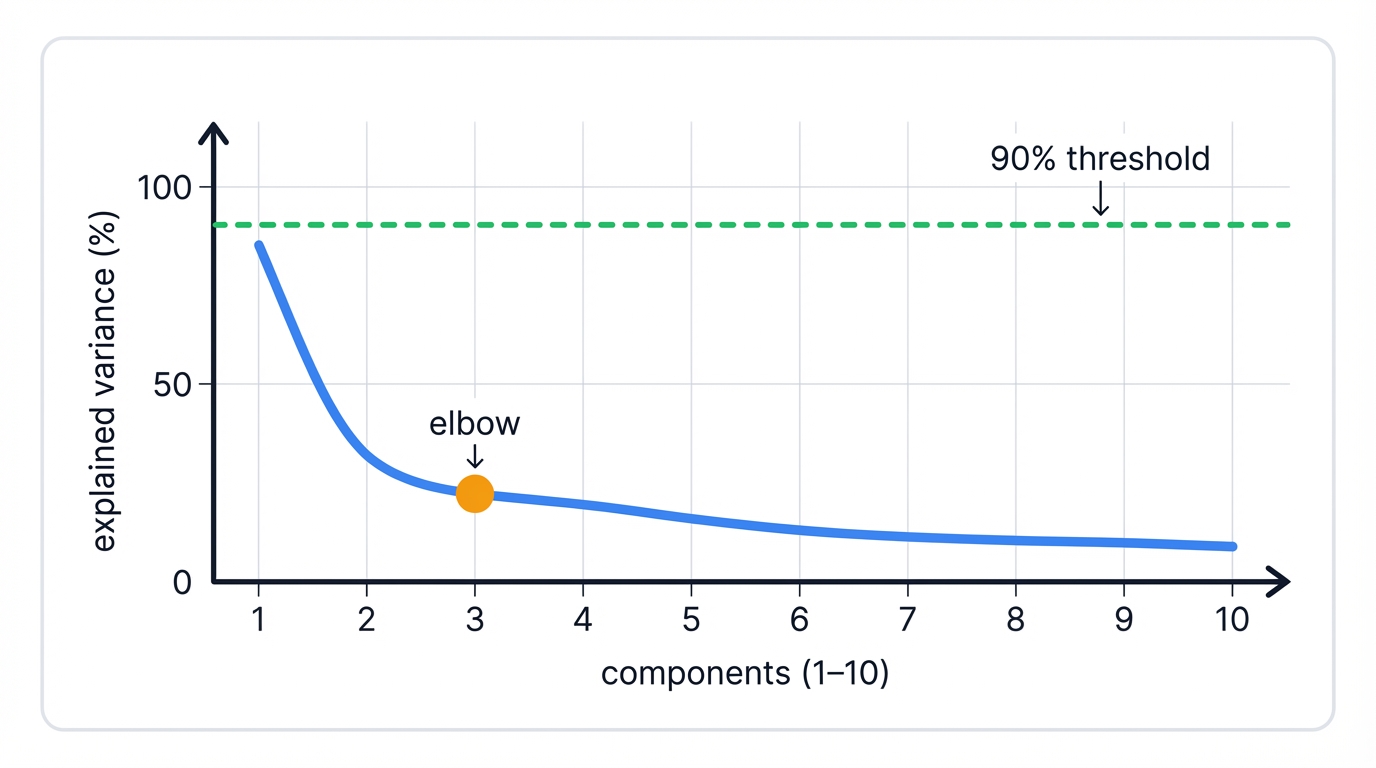
The explained variance threshold gives you a simple target. Decide what percentage of total variation you want to preserve—typically 80-95%—then keep enough components to hit that threshold:
cumulative_variance = np.cumsum(pca.explained_variance_ratio_)
n_components = np.argmax(cumulative_variance >= 0.95) + 1
The elbow method relies on visual inspection. Plot explained variance versus component number. Look for the bend where the curve levels off—where adding more components yields diminishing returns. Components before the elbow capture signal. Components after the elbow mostly capture noise.
Scree plots show eigenvalues directly. Watch for the point where eigenvalues flatten into a plateau of small, roughly equal values. Those small eigenvalues represent noise dimensions you can safely discard.
Working Example: Component Selection Strategies
import numpy as np
import matplotlib.pyplot as plt
from sklearn.decomposition import PCA
from sklearn.datasets import make_classification
from sklearn.preprocessing import StandardScaler

# Generate complex synthetic dataset
np.random.seed(42)
X, y = make_classification(n_samples=1000, n_features=50, n_informative=10,
                          n_redundant=10, n_clusters_per_class=1, random_state=42)

print("Component Selection Strategy Comparison")
print("=" * 40)

# Standardize the data
scaler = StandardScaler()
X_scaled = scaler.fit_transform(X)

# Fit PCA with all components
pca_full = PCA()
pca_full.fit(X_scaled)

print(f"Original data: {X.shape[1]} features")
print(f"Total variance: {np.sum(pca_full.explained_variance_):.3f}")

# Strategy 1: Explained Variance Threshold
thresholds = [0.80, 0.85, 0.90, 0.95, 0.99]
print(f"\nStrategy 1: Explained Variance Threshold")
print("-" * 35)

for threshold in thresholds:
    cumulative_var = np.cumsum(pca_full.explained_variance_ratio_)
    n_components = np.argmax(cumulative_var >= threshold) + 1
    actual_variance = cumulative_var[n_components - 1]

    print(f"  {threshold:.0%} threshold: {n_components:2d} components "
          f"(actual: {actual_variance:.1%})")

# Strategy 2: Elbow Method
print(f"\nStrategy 2: Elbow Method Analysis")
print("-" * 30)

# Calculate second derivative to find elbow
explained_var = pca_full.explained_variance_ratio_
first_derivative = np.diff(explained_var)
second_derivative = np.diff(first_derivative)

# Find point of maximum curvature
elbow_point = np.argmax(second_derivative) + 2  # +2 due to double differencing
print(f"  Elbow point detected at component: {elbow_point}")
print(f"  Variance explained by elbow point: {np.sum(explained_var[:elbow_point]):.1%}")

# Strategy 3: Kaiser Criterion (eigenvalues > 1)
print(f"\nStrategy 3: Kaiser Criterion (eigenvalues > 1)")
print("-" * 40)

eigenvalues_gt_1 = np.sum(pca_full.explained_variance_ > 1)
print(f"  Components with eigenvalue > 1: {eigenvalues_gt_1}")
print(f"  Variance explained: {np.sum(explained_var[:eigenvalues_gt_1]):.1%}")

# Strategy 4: Parallel Analysis (randomized baseline)
print(f"\nStrategy 4: Parallel Analysis")
print("-" * 25)

n_simulations = 100
random_eigenvalues = []

for _ in range(n_simulations):
    # Generate random data with same dimensions
    X_random = np.random.randn(*X_scaled.shape)
    pca_random = PCA()
    pca_random.fit(X_random)
    random_eigenvalues.append(pca_random.explained_variance_)

# Average eigenvalues from random data
mean_random_eigenvalues = np.mean(random_eigenvalues, axis=0)

# Find components where real eigenvalues exceed random baseline
significant_components = np.sum(pca_full.explained_variance_ > mean_random_eigenvalues)
print(f"  Components above random baseline: {significant_components}")
print(f"  Variance explained: {np.sum(explained_var[:significant_components]):.1%}")

# Visualization
fig, ((ax1, ax2), (ax3, ax4)) = plt.subplots(2, 2, figsize=(15, 12))

# Plot 1: Scree plot
components = range(1, min(21, len(explained_var) + 1))
ax1.plot(components, explained_var[:20], 'bo-', linewidth=2, markersize=6)
ax1.axvline(elbow_point, color='red', linestyle='--', label=f'Elbow (PC{elbow_point})')
ax1.set_xlabel('Principal Component')
ax1.set_ylabel('Explained Variance Ratio')
ax1.set_title('Scree Plot - Individual Components')
ax1.grid(True, alpha=0.3)
ax1.legend()

# Plot 2: Cumulative explained variance
cumulative_var = np.cumsum(explained_var)
ax2.plot(components, cumulative_var[:20], 'go-', linewidth=2, markersize=6)
for threshold in [0.8, 0.9, 0.95]:
    n_comp = np.argmax(cumulative_var >= threshold) + 1
    ax2.axhline(threshold, color='red', linestyle='--', alpha=0.7)
    ax2.axvline(n_comp, color='red', linestyle='--', alpha=0.7)
    ax2.text(n_comp + 0.5, threshold + 0.01, f'{threshold:.0%}\n({n_comp} PCs)',
             fontsize=8, ha='left')

ax2.set_xlabel('Principal Component')
ax2.set_ylabel('Cumulative Explained Variance')
ax2.set_title('Cumulative Explained Variance')
ax2.grid(True, alpha=0.3)

# Plot 3: Eigenvalue comparison (Kaiser + Parallel Analysis)
ax3.plot(components, pca_full.explained_variance_[:20], 'bo-',
         label='Actual Eigenvalues', linewidth=2)
ax3.plot(components, mean_random_eigenvalues[:20], 'ro-',
         label='Random Baseline', linewidth=2)
ax3.axhline(1, color='green', linestyle='--', label='Kaiser Criterion (λ=1)')
ax3.set_xlabel('Principal Component')
ax3.set_ylabel('Eigenvalue')
ax3.set_title('Eigenvalue Comparison')
ax3.legend()
ax3.grid(True, alpha=0.3)

# Plot 4: Component selection comparison
methods = ['80%', '85%', '90%', '95%', '99%', 'Elbow', 'Kaiser', 'Parallel']
n_components_methods = []

for threshold in [0.8, 0.85, 0.9, 0.95, 0.99]:
    n_comp = np.argmax(cumulative_var >= threshold) + 1
    n_components_methods.append(n_comp)

n_components_methods.extend([elbow_point, eigenvalues_gt_1, significant_components])

colors = ['skyblue'] * 5 + ['orange', 'green', 'purple']
bars = ax4.bar(methods, n_components_methods, color=colors, alpha=0.7)
ax4.set_ylabel('Number of Components')
ax4.set_title('Component Selection Method Comparison')
ax4.grid(True, alpha=0.3, axis='y')

# Add value labels on bars
for bar, n_comp in zip(bars, n_components_methods):
    height = bar.get_height()
    ax4.text(bar.get_x() + bar.get_width()/2., height + 0.5, f'{int(n_comp)}',
             ha='center', va='bottom', fontweight='bold')

plt.xticks(rotation=45)
plt.tight_layout()
plt.show()

# Recommendations
print(f"\n" + "="*50)
print("COMPONENT SELECTION RECOMMENDATIONS")
print("="*50)

print(f"Based on the analysis:")
print(f"  • Conservative approach (95% variance): {np.argmax(cumulative_var >= 0.95) + 1} components")
print(f"  • Balanced approach (90% variance): {np.argmax(cumulative_var >= 0.90) + 1} components")
print(f"  • Statistical approach (Parallel Analysis): {significant_components} components")
print(f"  • Elbow method suggests: {elbow_point} components")

# Final recommendation
recommended = np.argmax(cumulative_var >= 0.90) + 1
print(f"\nRECOMMENDED: {recommended} components")
print(f"  - Captures {cumulative_var[recommended-1]:.1%} of variance")
print(f"  - Reduces dimensionality by {(1 - recommended/X.shape[1]):.1%}")
print(f"  - Good balance of information retention and complexity reduction")
3.3 Interpreting Principal Components
Principal components combine your original features using specific weights. Understanding these combinations—interpreting what each component represents—validates your analysis and reveals insights about your data's underlying structure.
Component loadings show you exactly how PCA builds each component from your original features. High absolute loading values mean that feature contributes strongly to that component. Look at the top loadings to understand what each principal component captures—is it size? Color? Temperature? Financial risk? The loadings tell you.
Biplot visualization overlays two things: your data points projected onto the first two principal components, and vectors showing how original features contribute to those components. Points that cluster together are similar in PC space. Feature vectors pointing in the same direction correlate with each other. Long vectors indicate features that vary substantially.
Feature contributions quantify each variable's importance for explaining variance captured by each component. Calculate the squared loading value and you get that feature's contribution to the component's variance. Sum these across the components you keep, and you can identify which original features drive your reduced representation.
4. PCA + Hierarchical Clustering: The Complete Pipeline
PCA and hierarchical clustering form a natural partnership. PCA handles the dimensionality problem, clustering builds the tree structure that reveals your data's organization, and together they transform impossible high-dimensional clustering into tractable analysis with interpretable results.
4.1 The Complete Workflow
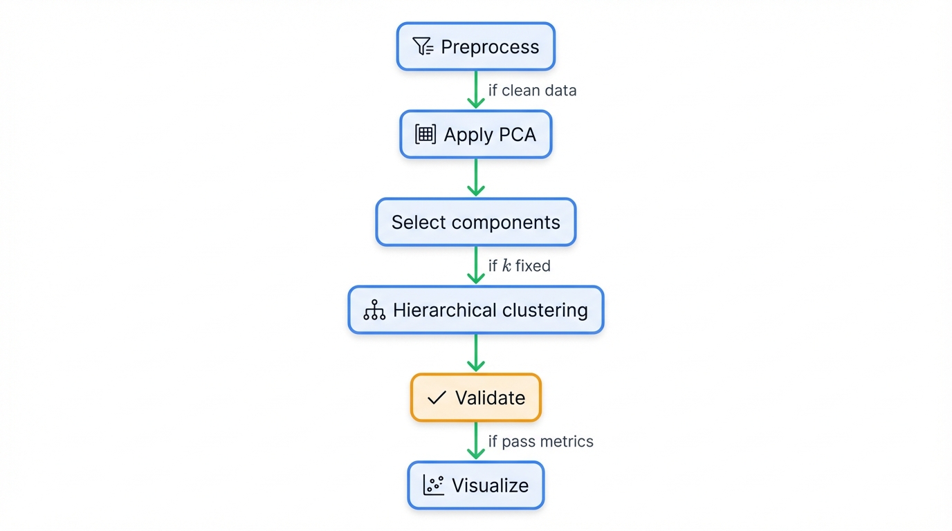
Six stages transform raw data into clustered insights:
- Preprocess: Clean your data ruthlessly—handle missing values, remove outliers, and scale features to equal footing
- Apply PCA: Reduce dimensionality while preserving the variation that matters
- Select Components: Choose how many dimensions to keep using variance thresholds or cross-validation
- Hierarchical Clustering: Build your dendrogram in the compressed space where distances mean something
- Validate Results: Test cluster quality using silhouette scores and domain knowledge
- Visualize: Plot your clusters in 2D or 3D PC space and examine the dendrogram structure
Working Example: Complete PCA + Clustering Pipeline
import numpy as np
import matplotlib.pyplot as plt
import seaborn as sns
from sklearn.datasets import load_digits, make_blobs
from sklearn.preprocessing import StandardScaler
from sklearn.decomposition import PCA
from scipy.cluster.hierarchy import linkage, dendrogram, fcluster
from scipy.spatial.distance import pdist
from sklearn.metrics import adjusted_rand_score, silhouette_score
import pandas as pd

print("COMPLETE PCA + HIERARCHICAL CLUSTERING PIPELINE")
print("=" * 52)

# Load a real high-dimensional dataset (handwritten digits)
digits = load_digits()
X, y_true = digits.data, digits.target

print(f"Dataset: Handwritten digits")
print(f"  Original shape: {X.shape}")
print(f"  Features: {X.shape[1]} pixel values (8x8 images)")
print(f"  Classes: {len(np.unique(y_true))} digit classes (0-9)")
print(f"  Samples per class: {np.bincount(y_true)}")

# Step 1: Data Preprocessing
print(f"\nStep 1: Data Preprocessing")
print("-" * 25)

# Check for missing values
print(f"  Missing values: {np.sum(np.isnan(X))}")

# Standardize the features
scaler = StandardScaler()
X_scaled = scaler.fit_transform(X)

print(f"  Data standardized: mean ≈ 0, std ≈ 1")
print(f"  Feature means: {np.mean(X_scaled, axis=0)[:5]}...")
print(f"  Feature stds: {np.std(X_scaled, axis=0)[:5]}...")

# Step 2: PCA Analysis
print(f"\nStep 2: Principal Component Analysis")
print("-" * 35)

# Fit PCA with all components first
pca_full = PCA()
pca_full.fit(X_scaled)

# Analyze explained variance
cumulative_variance = np.cumsum(pca_full.explained_variance_ratio_)

# Find optimal number of components (95% variance)
n_components_95 = np.argmax(cumulative_variance >= 0.95) + 1
n_components_90 = np.argmax(cumulative_variance >= 0.90) + 1

print(f"  Total components available: {len(pca_full.components_)}")
print(f"  Components for 90% variance: {n_components_90}")
print(f"  Components for 95% variance: {n_components_95}")
print(f"  Dimensionality reduction: {X.shape[1]} → {n_components_95} features")

# Apply PCA with selected components
pca = PCA(n_components=n_components_95)
X_pca = pca.fit_transform(X_scaled)

print(f"  Final PCA shape: {X_pca.shape}")
print(f"  Variance explained: {np.sum(pca.explained_variance_ratio_):.1%}")

# Step 3: Hierarchical Clustering in PC Space
print(f"\nStep 3: Hierarchical Clustering in PC Space")
print("-" * 43)

# Test different linkage methods
linkage_methods = ['ward', 'complete', 'average', 'single']
clustering_results = {}

for method in linkage_methods:
    print(f"\n  Testing {method.upper()} linkage:")

    # Perform hierarchical clustering
    Z = linkage(X_pca, method=method)

    # Get clusters (using true number of classes as reference)
    n_clusters = len(np.unique(y_true))
    cluster_labels = fcluster(Z, n_clusters, criterion='maxclust')

    # Evaluate clustering quality
    ari = adjusted_rand_score(y_true, cluster_labels)
    silhouette = silhouette_score(X_pca, cluster_labels)

    clustering_results[method] = {
        'linkage_matrix': Z,
        'labels': cluster_labels,
        'ari': ari,
        'silhouette': silhouette,
        'n_clusters': len(np.unique(cluster_labels))
    }

    print(f"    Clusters found: {len(np.unique(cluster_labels))}")
    print(f"    Adjusted Rand Index: {ari:.3f}")
    print(f"    Silhouette Score: {silhouette:.3f}")

# Step 4: Select Best Method
print(f"\nStep 4: Method Selection")
print("-" * 22)

best_method = max(clustering_results.keys(),
                 key=lambda x: clustering_results[x]['ari'])
best_result = clustering_results[best_method]

print(f"  Best method: {best_method.upper()} linkage")
print(f"  Best ARI: {best_result['ari']:.3f}")
print(f"  Best Silhouette: {best_result['silhouette']:.3f}")

# Step 5: Detailed Analysis of Best Result
print(f"\nStep 5: Detailed Analysis of Best Result")
print("-" * 38)

best_labels = best_result['labels']

# Analyze cluster composition
print(f"  Cluster composition analysis:")
for cluster_id in np.unique(best_labels):
    cluster_mask = best_labels == cluster_id
    cluster_true_labels = y_true[cluster_mask]
    most_common_digit = np.argmax(np.bincount(cluster_true_labels))
    purity = np.sum(cluster_true_labels == most_common_digit) / len(cluster_true_labels)

    print(f"    Cluster {cluster_id}: {np.sum(cluster_mask):3d} samples, "
          f"mainly digit {most_common_digit} ({purity:.1%} purity)")

# Step 6: Visualization
print(f"\nStep 6: Visualization")
print("-" * 18)

fig, axes = plt.subplots(2, 3, figsize=(18, 12))

# Plot 1: Explained variance
ax1 = axes[0, 0]
components_range = range(1, min(21, len(pca_full.explained_variance_ratio_) + 1))
ax1.plot(components_range, pca_full.explained_variance_ratio_[:20], 'bo-')
ax1.axvline(n_components_95, color='red', linestyle='--',
           label=f'95% variance ({n_components_95} PCs)')
ax1.set_xlabel('Principal Component')
ax1.set_ylabel('Explained Variance Ratio')
ax1.set_title('PCA Scree Plot')
ax1.legend()
ax1.grid(True, alpha=0.3)

# Plot 2: Cumulative variance
ax2 = axes[0, 1]
ax2.plot(components_range, cumulative_variance[:20], 'go-')
ax2.axhline(0.95, color='red', linestyle='--', alpha=0.7)
ax2.axvline(n_components_95, color='red', linestyle='--', alpha=0.7)
ax2.set_xlabel('Principal Component')
ax2.set_ylabel('Cumulative Variance Explained')
ax2.set_title('Cumulative Explained Variance')
ax2.grid(True, alpha=0.3)

# Plot 3: Data in PC space (first 2 components) - True labels
ax3 = axes[0, 2]
scatter = ax3.scatter(X_pca[:, 0], X_pca[:, 1], c=y_true, cmap='tab10', alpha=0.7)
ax3.set_xlabel(f'PC1 ({pca.explained_variance_ratio_[0]:.1%} variance)')
ax3.set_ylabel(f'PC2 ({pca.explained_variance_ratio_[1]:.1%} variance)')
ax3.set_title('Data in PC Space - True Labels')
plt.colorbar(scatter, ax=ax3)

# Plot 4: Data in PC space - Cluster labels
ax4 = axes[1, 0]
scatter2 = ax4.scatter(X_pca[:, 0], X_pca[:, 1], c=best_labels, cmap='viridis', alpha=0.7)
ax4.set_xlabel(f'PC1 ({pca.explained_variance_ratio_[0]:.1%} variance)')
ax4.set_ylabel(f'PC2 ({pca.explained_variance_ratio_[1]:.1%} variance)')
ax4.set_title(f'Data in PC Space - {best_method.title()} Clusters')
plt.colorbar(scatter2, ax=ax4)

# Plot 5: Dendrogram
ax5 = axes[1, 1]
# Sample subset for cleaner dendrogram
sample_indices = np.random.choice(len(X_pca), 100, replace=False)
Z_sample = linkage(X_pca[sample_indices], method=best_method)
dendrogram(Z_sample, ax=ax5, leaf_rotation=90, leaf_font_size=8)
ax5.set_title(f'{best_method.title()} Linkage Dendrogram (100 samples)')

# Plot 6: Clustering method comparison
ax6 = axes[1, 2]
methods = list(clustering_results.keys())
ari_scores = [clustering_results[m]['ari'] for m in methods]
sil_scores = [clustering_results[m]['silhouette'] for m in methods]

x = np.arange(len(methods))
width = 0.35

bars1 = ax6.bar(x - width/2, ari_scores, width, label='ARI', alpha=0.7)
bars2 = ax6.bar(x + width/2, sil_scores, width, label='Silhouette', alpha=0.7)

ax6.set_xlabel('Linkage Method')
ax6.set_ylabel('Score')
ax6.set_title('Clustering Method Comparison')
ax6.set_xticks(x)
ax6.set_xticklabels([m.title() for m in methods])
ax6.legend()
ax6.grid(True, alpha=0.3, axis='y')

# Add value labels on bars
for bars in [bars1, bars2]:
    for bar in bars:
        height = bar.get_height()
        ax6.text(bar.get_x() + bar.get_width()/2., height + 0.01, f'{height:.3f}',
                ha='center', va='bottom', fontsize=8)

plt.tight_layout()
plt.show()

# Step 7: Final Summary
print(f"\n" + "="*60)
print("PIPELINE EXECUTION SUMMARY")
print("="*60)

print(f"✅ Data preprocessing: {X.shape[0]} samples, {X.shape[1]} → {X_pca.shape[1]} features")
print(f"✅ PCA dimensionality reduction: {(1-X_pca.shape[1]/X.shape[1])*100:.0f}% reduction")
print(f"✅ Variance preservation: {np.sum(pca.explained_variance_ratio_)*100:.1f}%")
print(f"✅ Best clustering method: {best_method.upper()} linkage")
print(f"✅ Clustering quality: ARI = {best_result['ari']:.3f}")
print(f"✅ Internal validity: Silhouette = {best_result['silhouette']:.3f}")

print(f"\nKey Benefits Achieved:")
print(f"  • Made high-dimensional clustering computationally feasible")
print(f"  • Preserved {np.sum(pca.explained_variance_ratio_)*100:.1f}% of data variation")
print(f"  • Reduced noise and irrelevant features")
print(f"  • Enabled meaningful visualization in 2D/3D")
print(f"  • Achieved reasonable clustering quality on complex data")

print(f"\nRecommendations:")
print(f"  • Use {n_components_95} principal components for this type of data")
print(f"  • Apply {best_method} linkage for similar clustering tasks")
print(f"  • Consider ensemble methods for even better results")
print(f"  • Validate on additional datasets to confirm generalizability")
4.2 Benefits and Limitations
Important Consideration: This approach delivers major advantages, but you need to understand where it fails and what assumptions it makes before you deploy it on production data.
Benefits of PCA + Clustering:
- Computational efficiency explodes—clustering in 20 dimensions runs orders of magnitude faster than clustering in 2000
- Noise reduction happens automatically—PCA filters out the random fluctuations trapped in low-variance components
- Visualization becomes possible—you can actually see your clusters in 2D or 3D plots instead of trusting black-box algorithms
- Interpretability improves when principal components align with meaningful concepts in your domain
Limitations to Consider:
- Linear assumption restricts you—PCA only captures linear combinations of features, missing complex nonlinear patterns
- Information loss is guaranteed—you're throwing away variance, and sometimes that discarded variance contains signal
- Component interpretability fails frequently—PCs often mix features in ways that don't match human concepts
- Preprocessing sensitivity means results shift dramatically based on how you scale and normalize your features
5. Advanced Techniques and Variations
Standard PCA handles linear relationships in numeric data. But what about curved manifolds? What about datasets too large for memory? What about components you can actually interpret? Advanced techniques extend PCA's reach beyond its original scope.
5.1 Kernel PCA: Nonlinear Dimensionality Reduction
Linear PCA misses curved patterns. Your data might lie on a twisted manifold in high-dimensional space, and standard PCA tries to flatten it with a straight projection, destroying the structure you need to preserve. Kernel PCA fixes this using the kernel trick—it implicitly maps your data to a higher-dimensional space where the curved pattern becomes linear, then applies PCA there, all without ever explicitly computing the high-dimensional coordinates.
Three popular kernels unlock different pattern types:
- RBF (Radial Basis Function) captures local similarities, creating smooth nonlinear embeddings that preserve neighborhood structure
- Polynomial finds relationships where features combine multiplicatively rather than additively
- Sigmoid mimics neural network activations, discovering patterns similar to what a simple neural network would learn
from sklearn.decomposition import KernelPCA

# RBF kernel for nonlinear relationships
kpca = KernelPCA(n_components=2, kernel='rbf', gamma=0.1)
X_kpca = kpca.fit_transform(X_scaled)
5.2 Sparse PCA: Interpretable Components
Standard PCA creates dense components. Every principal component uses every feature with some nonzero weight, producing linear combinations that mix dozens or hundreds of variables together in ways that defy interpretation. Sparse PCA adds a penalty that drives most weights to exactly zero, creating components that depend on just a small subset of features. You sacrifice some optimality—sparse PCA doesn't capture quite as much variance as standard PCA—but you gain interpretability that makes the tradeoff worthwhile in many applications.
from sklearn.decomposition import SparsePCA

spca = SparsePCA(n_components=5, alpha=0.1)
X_sparse = spca.fit_transform(X_scaled)

# Components use fewer features
print("Sparse PCA component sparsity:")
for i, component in enumerate(spca.components_):
    non_zero = np.sum(np.abs(component) > 1e-6)
    print(f"  PC{i+1}: {non_zero}/{len(component)} features used")
5.3 Incremental PCA: Handling Large Datasets
Standard PCA demands that your entire dataset fits in memory simultaneously. It needs to compute the covariance matrix across all samples at once, which becomes impossible when you're working with millions of observations or when each sample contains high-resolution images. Incremental PCA processes data in batches, computing running statistics that converge to the same principal components standard PCA would find, but using only a fraction of the memory.
from sklearn.decomposition import IncrementalPCA

# Process large dataset in batches
ipca = IncrementalPCA(n_components=50, batch_size=1000)

# Fit incrementally
for batch in batches:
    ipca.partial_fit(batch)

# Transform data
X_incremental = ipca.transform(X_scaled)
6. Evaluation and Validation
Running PCA and clustering is easy. Validating that your results make sense? That requires rigorous evaluation of both the dimensionality reduction quality and the clustering performance, using metrics that reveal whether you've discovered genuine structure or fitted to noise.
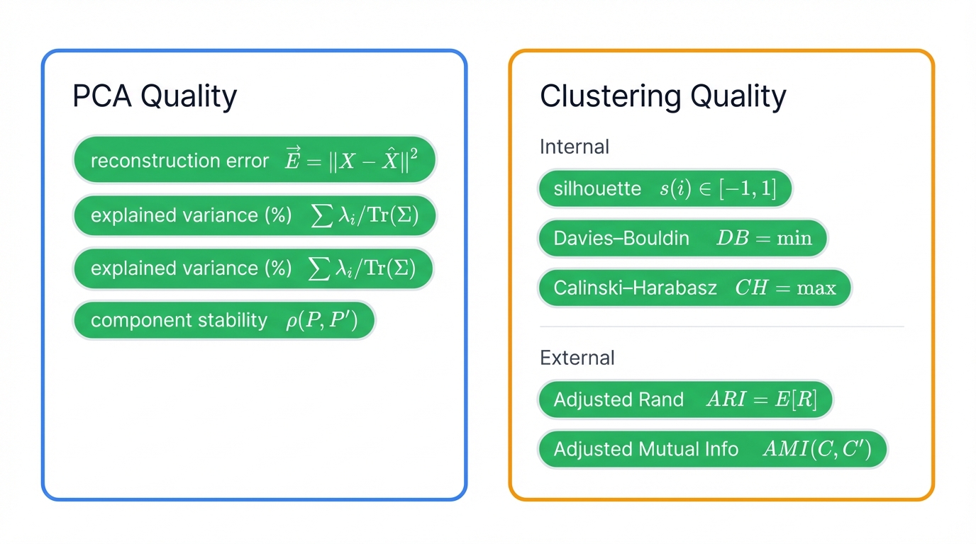
6.1 PCA Quality Assessment
Reconstruction error quantifies information loss. Project your data into PC space, then project back to the original feature space. Compare the reconstructed data to the original. Mean squared error tells you how much detail you lost:
X_reconstructed = pca.inverse_transform(X_pca)
reconstruction_error = np.mean((X_scaled - X_reconstructed) ** 2)
print(f"Reconstruction error: {reconstruction_error:.6f}")
Explained variance ratio shows what fraction of total variation each component captures. Look for components that explain substantial variance—say, more than 5% individually. Cumulative explained variance tells you how many components you need to hit your target threshold, whether that's 80%, 90%, or 95% of total variation.
Component stability tests reliability. Take random subsets of your data, apply PCA to each subset, and compare the resulting components. Stable components point in similar directions across subsets, indicating genuine patterns. Unstable components rotate wildly, suggesting you're fitting to noise that changes with each random sample.
6.2 Clustering Quality Metrics
Internal Metrics work without ground truth labels:
- Silhouette Score ranges from -1 to +1—higher values mean points are close to their cluster center and far from other clusters
- Davies-Bouldin Index measures cluster separation—lower values indicate better-separated, more compact clusters
- Calinski-Harabasz Index rewards compact, well-separated clusters—higher values suggest better clustering
External Metrics compare against known labels:
- Adjusted Rand Index measures agreement with true labels, correcting for chance—values near 1 indicate strong agreement
- Adjusted Mutual Information quantifies shared information between cluster assignments and true labels, accounting for random agreement
6.3 Validation Strategies
Cross-validation adapts to unsupervised learning. Split your data into folds. Fit PCA on the training folds, then transform the held-out fold and cluster it. Repeat across all folds. Consistent cluster structures across folds indicate stable, reproducible patterns rather than artifacts of one particular data split.
Bootstrap validation tests robustness. Generate bootstrap samples by sampling with replacement from your original data. Apply the complete PCA + clustering pipeline to each bootstrap sample. Measure how much cluster assignments vary—stable assignments suggest real structure, while high variability indicates you're clustering noise.
Parameter sensitivity analysis reveals whether your findings depend critically on arbitrary choices. Try different numbers of components. Test various linkage methods. Adjust preprocessing steps. Robust discoveries persist across reasonable parameter ranges, while fragile results collapse when you tweak the knobs.
7. Real-World Applications and Case Studies
PCA + hierarchical clustering solves real problems across industries. From genomics to finance, from computer vision to customer analytics, this pipeline transforms overwhelming complexity into actionable insights.
7.1 Genomics and Bioinformatics
Gene expression analysis drowns in dimensions. RNA-seq experiments measure 20,000+ genes simultaneously across hundreds of patient samples, creating datasets where the number of features vastly exceeds the number of observations. Standard statistical methods fail completely. PCA compresses this complexity into 10-50 principal components that capture biological variation while discarding technical noise, then hierarchical clustering reveals:
- Disease subtypes that respond differently to treatment, enabling personalized medicine strategies
- Gene modules that activate together, suggesting shared regulatory mechanisms and functional relationships
- Batch effects and quality control issues that require correction before biological interpretation
Single-cell RNA sequencing pushes scale to extremes. Modern scRNA-seq datasets contain millions of individual cells, each measured across thousands of genes, creating computational challenges that make PCA preprocessing essential rather than optional. Researchers apply PCA to reduce dimensions, then cluster in PC space to identify distinct cell types, developmental stages, and disease-specific cell populations that drive pathology.
7.2 Image Analysis and Computer Vision
Face recognition powered some of PCA's earliest practical successes. The eigenfaces approach represents facial images as linear combinations of principal component "eigenfaces," creating compact representations that enable fast matching and recognition. Each image becomes a point in a low-dimensional PC space, and hierarchical clustering groups similar faces together based on lighting, pose, and identity.
Medical image analysis leverages PCA to handle the dimensionality explosion in radiological imaging, pathology slides, and microscopy data. A single MRI scan contains millions of voxels, a whole-slide pathology image contains billions of pixels, yet PCA combined with clustering can identify:
- Tumor subtypes with distinct imaging signatures that predict treatment response
- Disease progression patterns that cluster patients into risk groups
- Quality control clusters that separate good images from artifacts requiring re-acquisition
7.3 Market Research and Customer Analytics
Customer segmentation drives revenue in e-commerce. Modern platforms track hundreds of behavioral features per customer—pages viewed, products clicked, time on site, purchase frequency, cart abandonment patterns, email engagement, and social media interactions. PCA reduces this tsunami of metrics to a handful of interpretable dimensions like "engagement level" and "price sensitivity," then clustering reveals distinct customer segments that marketing teams can target:
- High-value loyalists who respond to premium products and loyalty programs
- Bargain hunters who need discount triggers to convert
- Window shoppers who browse extensively but rarely purchase, requiring different engagement strategies
Survey analysis in market research faces the curse of dimensionality from Likert-scale questions. A comprehensive market survey might include 50-100 rating questions, creating challenges for direct analysis. PCA discovers underlying attitude dimensions that multiple questions measure—like "brand affinity" or "price consciousness"—then hierarchical clustering groups respondents based on these latent attitudes rather than raw responses.
8. Common Pitfalls and How to Avoid Them
PCA + clustering can fail spectacularly when you violate its assumptions or skip critical preprocessing steps. Learn from others' mistakes before making them yourself.
8.1 Preprocessing Errors
Forgetting to scale destroys PCA results. Features with different measurement scales dominate the covariance matrix through magnitude alone, not through genuine importance. A feature measured in thousands overpowers one measured in decimals, regardless of which contains more information about cluster structure. Always use StandardScaler or similar normalization to give each feature equal standing.
Including irrelevant features pollutes your components. PCA tries to explain all variance, including meaningless noise from features that contain no signal about the structure you care about. Customer ID numbers, random identifier strings, and redundant derived features waste dimensions and dilute your principal components. Remove them before running PCA.
Ignoring missing values crashes your analysis. Eigendecomposition requires complete matrices—no gaps, no placeholders, no null values scattered through your data. You must either impute missing values using sophisticated methods that preserve statistical properties, or remove samples with incomplete data if your dataset is large enough to tolerate the loss.
8.2 Component Selection Errors
Arbitrary cutoffs waste information or include garbage. Blindly choosing "the first 10 components" ignores your data's actual structure. Maybe 5 components capture 95% of variance. Maybe you need 30 to hit that threshold. Use explained variance analysis, scree plots, and cross-validation to select numbers that match your data, not round numbers that match your intuition.
Overfitting to noise happens when you keep too many components. Those last few principal components with tiny eigenvalues? They often capture random fluctuations rather than genuine patterns. Including them in your clustering analysis adds noise that degrades performance. Balance information retention against noise reduction—90% explained variance often beats 99% when that last 9% is mostly measurement error.
8.3 Interpretation Mistakes
Over-interpreting components leads to false insights. Principal components are mathematical constructs optimized for variance capture, not meaningful domain concepts. PC1 might happen to align with "customer value" in one dataset, but in another it might be a meaningless mix of correlated noise. Always validate interpretations against domain knowledge and additional data before treating components as real phenomena.
Ignoring loadings blinds you to what drives each component. Component scores tell you where samples fall along each principal axis, but loadings reveal which original features define those axes. You need both for interpretation—scores show the what, loadings show the why, and together they complete the story of your data's structure.
9. Modern Alternatives and Future Directions
PCA remains foundational, taught in every machine learning course, deployed in thousands of production systems. But modern techniques address its limitations, handling nonlinear manifolds, preserving local structure, and learning representations that standard PCA misses.
9.1 Nonlinear Dimensionality Reduction
t-SNE creates stunning visualizations. t-Distributed Stochastic Neighbor Embedding excels at revealing cluster structure in 2D plots, preserving local neighborhoods while separating distant points. But it's terrible for clustering—the algorithm's stochastic nature means you get different results each run, and it distorts global structure in ways that break distance-based clustering algorithms. Use t-SNE for visualization after clustering, not before.
UMAP balances local and global structure better than alternatives. Uniform Manifold Approximation and Projection preserves both neighborhood relationships and broader data topology, making it genuinely useful for clustering preprocessing. It often outperforms PCA on datasets with nonlinear structure while remaining computationally tractable and producing stable, reproducible results.
Autoencoders learn nonlinear compressions through neural networks. You train an encoder network to compress high-dimensional inputs into low-dimensional "bottleneck" representations, then train a decoder network to reconstruct the original inputs from those representations. The bottleneck activations become your reduced-dimension features, capturing complex patterns that linear PCA cannot. But autoencoders require more data, more computation, and more hyperparameter tuning than PCA's clean mathematical solution.
9.2 Integrated Clustering Approaches
Deep clustering learns representations and cluster assignments simultaneously. Instead of the two-stage PCA-then-cluster pipeline, algorithms like Deep Embedded Clustering and Joint Unsupervised Learning train neural networks to optimize both dimensionality reduction and cluster quality in a single end-to-end framework. This joint optimization can discover representations specifically tailored for clustering rather than generic variance-maximizing PCA components.
Spectral clustering uses eigendecomposition differently than PCA. While PCA decomposes the covariance matrix, spectral clustering decomposes a similarity matrix constructed from pairwise distances or kernel functions. This approach often works better for data with non-convex cluster shapes that defeat hierarchical clustering's distance-based merging strategies.
9.3 Future Developments
Quantum computing looms on the distant horizon, promising revolutionary speedups for eigenvalue problems and optimization tasks that underlie both PCA and clustering. The combinatorial optimization problems at clustering's heart map naturally to quantum algorithms like QAOA and VQE. As quantum hardware matures beyond current noisy intermediate-scale quantum devices, we might see quantum-accelerated clustering on datasets with millions or billions of samples—problems completely intractable for classical computers. But practical quantum advantage remains years or decades away, so don't wait for quantum computers to solve today's clustering challenges.
10. A Curated Guide to Further Learning
You've seen the theory, worked through the code, and understood the pitfalls. Now go deeper. This section points you toward the foundational papers, practical tutorials, and benchmark datasets that will sharpen your skills and deepen your understanding of PCA and hierarchical clustering.
10.1 Seminal and Essential Academic Papers
Understanding the field requires reading its origins and evolution through key publications that shaped modern practice.
On Principal Component Analysis:
Pearson, K. (1901). "On Lines and Planes of Closest Fit to Systems of Points in Space." Philosophical Magazine. This started it all. Karl Pearson laid out the mathematical principles for finding the lines and planes that best fit a system of points, creating the foundation on which all PCA implementations build.
Hotelling, H. (1933). "Analysis of a Complex of Statistical Variables Into Principal Components." Journal of Educational Psychology. Harold Hotelling independently developed and formally named the technique, establishing it as a fundamental tool in statistical analysis that would outlive its original psychological applications.
Jolliffe, I. T. (2002). Principal Component Analysis. Springer. This comprehensive book stands as the definitive modern reference—theory, applications, interpretations, and extensions all in one authoritative source that belongs on every practitioner's shelf.
On Hierarchical Clustering:
Ward Jr, J. H. (1963). "Hierarchical grouping to optimize an objective function." Journal of the American Statistical Association. Joe Ward introduced the variance-minimizing linkage criterion that became the field's workhorse method, balancing cluster compactness against separation in ways that simple linkage methods miss.
Murtagh, F., & Contreras, P. (2012). "Algorithms for hierarchical clustering: an overview." WIREs Data Mining and Knowledge Discovery. This survey paper synthesizes decades of research, comparing algorithms and linkage criteria with clarity that makes complex tradeoffs understandable.
On the Combined PCA + Clustering Approach:
Yeung, K. Y., & Ruzzo, W. L. (2001). "Principal component analysis for clustering gene expression data." Bioinformatics. Every practitioner needs this paper's wisdom. It provides rigorous empirical evaluation showing when PCA preprocessing helps clustering performance and, critically, when it actually makes results worse—essential knowledge for avoiding the pitfall of blind PCA application.
10.2 Recommended Tutorials, Courses, and Repositories
Theory becomes skill through practice. These resources offer structured learning paths, hands-on tutorials, and working code that transforms understanding into capability.
Online Courses: Coursera delivers structured education through courses like "Clustering Analysis" and "Cluster Analysis in Data Mining," which include dedicated modules on hierarchical clustering and PCA with graded exercises that force you to apply concepts rather than passively absorb them.
Tutorials and Documentation: The official scikit-learn documentation provides excellent user guides with working examples that you can run immediately. GeeksforGeeks and Towards Data Science host walkthrough articles that implement the complete pipeline step-by-step, explaining design decisions and debugging common errors along the way.
Code Repositories: Kaggle notebooks show real practitioners applying PCA + clustering to actual datasets with all the messy preprocessing and parameter tuning that textbooks skip. The "Clustering using K-Means, Hierarchical, PCA" notebook demonstrates complete workflows on NGO data with detailed explanations. GitHub repositories dedicated to hierarchical clustering projects offer well-documented implementations you can fork and adapt to your own problems.
10.3 Benchmarking Datasets
Testing your implementations requires standard datasets that let you compare results against published baselines. The UCI Machine Learning Repository hosts the classics:
Iris Dataset: Small and clean, containing 150 iris flower samples from three species described by four features. It's perfect for initial validation—small enough to understand completely, structured enough to show clear clusters, and simple enough that you can visualize results and debug algorithms without drowning in complexity.
Wine Dataset: Chemical analysis of 178 Italian wines from three cultivars, measured across 13 continuous features. This dataset tests PCA's ability to reduce correlated chemical measurements into interpretable components while revealing the natural grouping structure that exists in the original high-dimensional space.
Breast Cancer Wisconsin (Diagnostic) Dataset: Real medical data with 569 instances and 30 continuous features computed from breast mass images. Originally designed for classification, it serves as an excellent clustering benchmark that tests your pipeline on realistic data with clinical importance and complex feature relationships.
10.4 Modern ML Operations (MLOps) Integration
Production environments demand reproducibility. One-off analyses in notebooks give way to automated pipelines that run reliably on new data, track experiments rigorously, and integrate with broader ML systems seamlessly.
ML Pipelines: Kubeflow Pipelines let you define each analysis stage—data ingestion, preprocessing, scaling, PCA, hierarchical clustering, and evaluation—as a containerized component. Chain these components into directed acyclic graphs that represent complete workflows. This modular architecture promotes reusability, makes debugging tractable, and enables you to re-run analyses on new data automatically without manual intervention.
Experiment Tracking: MLflow captures the iterative process of finding optimal parameters. Log every pipeline run with its hyperparameters—number of components retained, linkage method chosen, scaling approach used. Track input data versions, evaluation metrics like Silhouette Score and Davies-Bouldin Index, and output artifacts including dendrogram plots and cluster assignments. This creates an auditable record that enables systematic comparison of different approaches and ensures full reproducibility when you need to recreate results months or years later.