Introduction: The Genesis of Machine Learning
The Perceptron changed everything. Not just an algorithm—a revolution. Computing would never think the same way again, and neither would artificial intelligence, because for the first time a machine could learn from experience by adjusting its own parameters rather than following rigid instructions programmed line by line. Psychologist Frank Rosenblatt invented this breakthrough in 1957, demonstrating that machines could adapt, evolve, and improve through data rather than through explicit human intervention at every step.
Key Concept: Understanding this foundational concept is essential for mastering the techniques discussed in this article.
Why does this matter? Because every neural network you encounter today—from the simplest classifier to the most sophisticated transformer powering modern language models—descends directly from this innovation. The Perceptron established the core principle that drives all machine learning: weights can change, boundaries can shift, and machines can learn.
This report explores the Perceptron from every angle, beginning with its fascinating history that stretches from early neuroscience through Rosenblatt's bold experiments to the media frenzy and subsequent controversy that nearly killed neural network research entirely. We break down its architecture piece by piece, revealing the elegant mathematics that power its predictions and learning mechanisms. Through concrete examples like modeling basic logic gates, we show exactly what the Perceptron can do and where it fails spectacularly. Finally, we examine the famous critique that exposed its fundamental limitations, the AI Winter that followed, and the eventual evolution into the Multi-Layer Perceptron that powers today's deep learning revolution.
The Perceptron didn't emerge from a vacuum. It crystallized from decades of interdisciplinary research aimed at one audacious goal: replicating the mechanisms of the human brain. Neuroscience provided the biological blueprint. Computer science supplied the simulation tools. Hardware engineering built the physical form. This interdisciplinary convergence still defines AI research today.
1.1 The Theoretical Precursors
Before computers could think, scientists needed to understand how neurons work. The breakthrough arrived in 1943. Neurophysiologist Warren McCulloch and mathematician Walter Pitts published "A Logical Calculus of the Ideas Immanent in Nervous Activity," introducing the first mathematical model of a biological neuron—now called the McCulloch-Pitts (MCP) neuron.
Simple. Elegant. Powerful. The model took binary inputs, summed them, and generated a binary output if the sum exceeded a threshold. Static, yes—the weights stayed fixed, the threshold required manual setting, and nothing learned or adapted. But it proved something revolutionary: brain function could be represented mathematically and electronically. This was the seed from which all artificial neurons would grow.
Five years later, psychologist Donald Hebb added the learning piece. His 1949 book, The Organization of Behavior, proposed a theory about how brains actually learn. The key idea? "Cells that fire together, wire together." When neurons activate simultaneously, their connections strengthen. This Hebbian learning principle linked brain activity directly to synaptic changes, offering the biological insight needed to create adaptive learning algorithms.
1.2 Frank Rosenblatt and the Invention of the Perceptron
Enter Frank Rosenblatt. A psychologist at Cornell Aeronautical Laboratory, he saw what others missed: the MCP neuron's rigidity could be transformed into flexibility. Instead of fixed connections, what if those connections could change? What if they could learn?
Rosenblatt aimed to build a machine that could see, recognize, and learn from its environment—like a brain does. In 1957, he described his invention in a technical report: "The Perceptron—a perceiving and recognizing automaton." Shortly after, he tested it on a computer. It worked. The system learned to distinguish patterns.
This leap from theory to working software marked a pivotal moment in AI history. Most importantly, Rosenblatt developed a systematic method for the machine to adjust itself, reducing errors in pattern recognition. He transformed a simple logic device into a learning machine.
1.3 The Mark I Perceptron: Hardware and Hype
Rosenblatt didn't stop at software. He wanted a physical machine. By 1958, the Mark I Perceptron existed: a hardware system built for image recognition featuring a 20x20 grid of 400 photocells acting as a "retina" connected to processing units.
The architecture comprised three unit types: Sensory (S) units received stimuli, Association (A) units processed signals, and Response (R) units produced the final output. Historic records document this elegant design that mirrored biological visual processing.
Then the hype machine cranked up. The Mark I sparked enormous public excitement and media frenzy, launching the classic technology hype cycle. A 1958 Navy press conference led to sensational coverage in The New York Times, which reported that the Navy expected the Perceptron to become "the embryo of an electronic computer that...will be able to walk, talk, see, write, reproduce itself and be conscious of its existence."
Walk. Talk. Be conscious. These wildly optimistic predictions triggered fierce controversy within the AI community and set impossibly high expectations. The gap between hype and reality would later prove catastrophic.
While journalists wrote breathless predictions, a classified project operated in the shadows. From 1963 to 1966, the U.S. National Photographic Interpretation Center (NPIC) ran a four-year program to develop Perceptron-based tools for analyzing satellite imagery. This early military application reveals a pattern that continues today: practical AI research funded by government and defense agencies, operating on a parallel, classified track away from public scrutiny.
The collision between public promises of human-like intelligence and later-discovered technical limitations would lead to a devastating backlash.
At its core, the Perceptron is a mathematical model of a biological neuron designed to capture one fundamental process: integrating signals and making a binary decision. Understanding this architecture reveals both its capabilities and its fatal limitations.
2.1 The Biological Analogy
Let's build intuition by grounding the Perceptron's components in their biological counterparts.
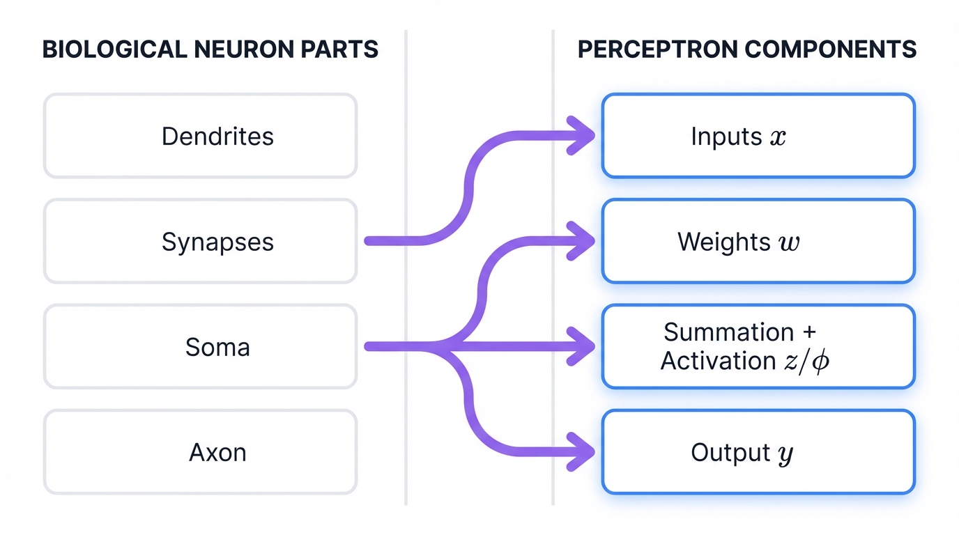
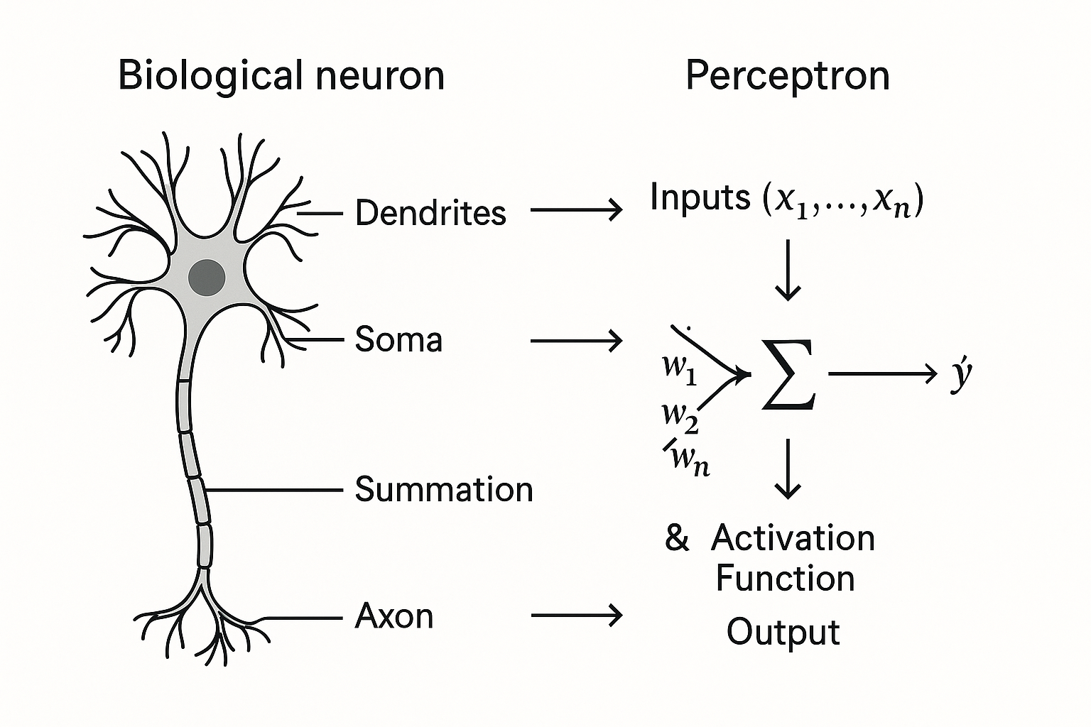
Dendrites receive signals from other neurons. In a Perceptron, these become Input Values (x).
Synapses modulate signal strength at connection points. This corresponds to Weights (w).
The Soma (cell body) aggregates signals and determines whether to fire. This maps to the Summation Function (z) and Activation Function.
The Axon transmits the final signal to other neurons if the threshold is met. This becomes the Perceptron's Output.
This biological analogy provides the conceptual scaffold for the formal mathematical description that follows.
2.2 Core Components and Mathematical Formulation
A single-layer Perceptron combines several key elements to process information and produce classifications.
Input Values (x): The features of a data point, represented as a numerical vector, $\mathbf{x}=[x_1, x_2, ..., x_n]$. The Perceptron processes real-valued inputs—a significant upgrade from the binary-only inputs of the McCulloch-Pitts neuron.
Weights (w): Each input feature $x_i$ connects to a real-valued weight $w_i$. These weights form a vector $\mathbf{w}=[w_1, w_2, ..., w_n]$ that signifies each input's importance in decision-making. The Perceptron learns these parameters from training data.
The Bias (b): Beyond weighted inputs, a scalar term called the bias, $b$, provides additional flexibility. The bias acts as an adjustable threshold, allowing the decision boundary to shift away from the feature space origin. A common mathematical convenience treats the bias as a weight $w_0$ corresponding to a constant input $x_0 = 1$, enabling the bias to learn alongside other weights.
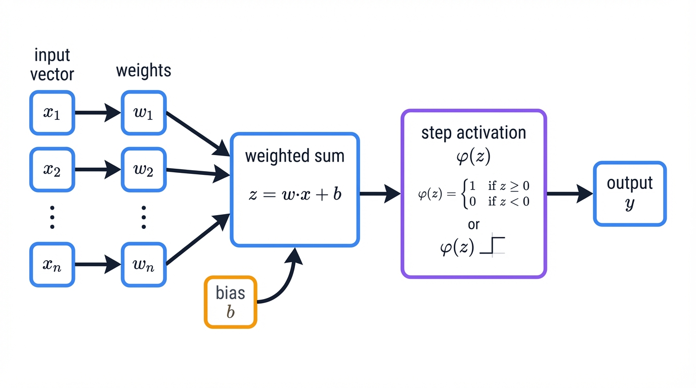
Summation Function (z): The Perceptron computes a weighted sum of its inputs—a linear aggregation calculated as the dot product of weight and input vectors, plus the bias term:
$$z = (w_1x_1 + w_2x_2 + \cdots + w_nx_n) + b = \mathbf{w} \cdot \mathbf{x} + b$$This linear combination forms the Perceptron's core computation.
Step Activation Function (φ): The weighted sum $z$ passes through a non-linear activation function to produce the final output. The classic Perceptron uses a Heaviside step function that mimics biological neuron "firing." If the weighted sum $z$ meets or exceeds a threshold (typically 0), the neuron fires and outputs 1; otherwise, it outputs 0 (or -1, depending on convention):
$$\text{output} = \phi(z) = \begin{cases} 1 & \text{if } z \geq 0 \\ 0 \text{ (or -1)} & \text{if } z < 0 \end{cases}$$This step function introduces decision-making capability into the model.
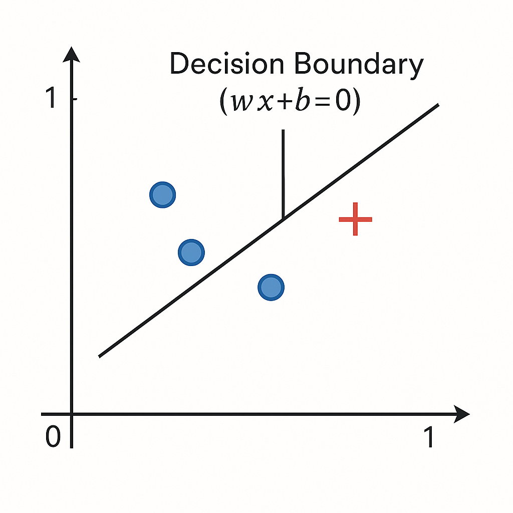
The Perceptron's architecture is fundamentally linear. The core computation—the weighted sum $z = \mathbf{w} \cdot \mathbf{x} + b$—defines a hyperplane in n-dimensional space. The step function uses this hyperplane to divide the entire feature space into two distinct half-spaces, one for each class.
This architectural design predetermines that a single-layer Perceptron can only learn linear decision boundaries. This inherent linearity creates both elegant simplicity and severe limitation.
The real innovation? The Perceptron learns. This learning involves two stages: the forward pass, where predictions happen, and the training phase, where internal weights adjust based on errors.
3.1 The Forward Pass: Making a Prediction
Once trained, a Perceptron classifies new, unseen data through a process called forward propagation. Straightforward. Sequential. Fast.
Input: Provide a new data point to the model as an input vector $\mathbf{x}$.
Weighted Sum: Calculate the weighted sum of inputs by computing the dot product with the learned weight vector $\mathbf{w}$ and adding the learned bias $b$: $z = \mathbf{w} \cdot \mathbf{x} + b$.
Activation: Pass the weighted sum $z$ through the step activation function $\phi$ to produce the final predicted class label, $\hat{y} = \phi(z)$.
This straightforward process makes prediction computationally inexpensive and blazingly fast.
3.2 The Perceptron Learning Rule
The heart of the Perceptron beats here: its learning algorithm. Simple. Intuitive. Elegant. The method adjusts weights based on prediction errors through supervised learning, requiring a training dataset with known correct labels.
The algorithm processes training data one example at a time, refining weights with each step. This exemplifies "online learning," where the model updates parameters after processing each individual training sample—perfect for large or streaming datasets.
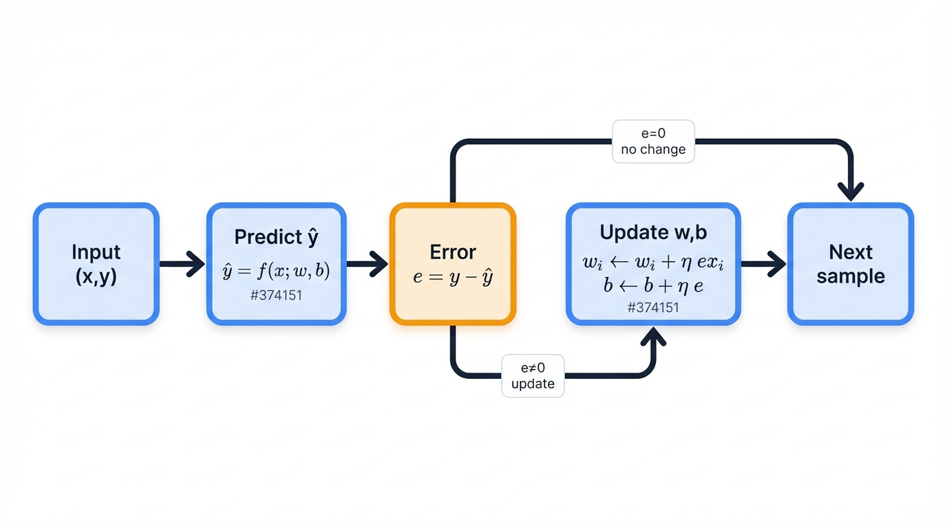
For each training example $(\mathbf{x},y)$, where $y$ is the true label:
Prediction: Perform a forward pass to obtain the predicted output, $\hat{y}$.
Error Calculation: Compute the error as the difference between the true label and predicted label: $\text{error} = y - \hat{y}$.
Weight Update: Adjust each weight $w_i$ and the bias $b$ according to the Perceptron learning rule:
$$w_i^{(\text{new})} = w_i^{(\text{old})} + \eta \cdot (y - \hat{y}) \cdot x_i$$ $$b^{(\text{new})} = b^{(\text{old})} + \eta \cdot (y - \hat{y})$$where $\eta$ is the learning rate.
The logic of this update rule? Beautiful simplicity.
If the prediction is correct, then $y - \hat{y} = 0$. Weights and bias remain unchanged. The model earns a reward for correctness: no alteration.
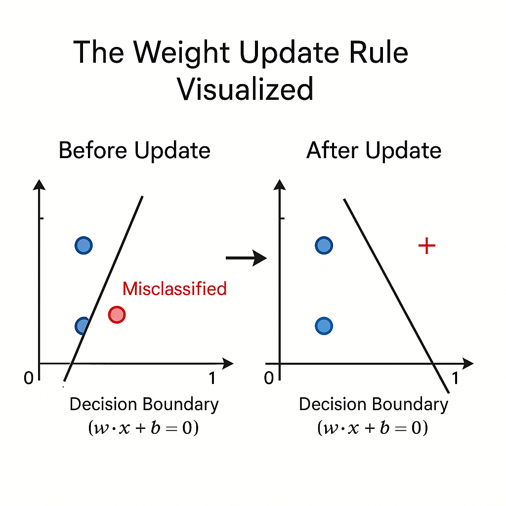
If the prediction is incorrect, weights shift in a direction that makes correct prediction more likely in the future.
False Negative: The model predicts 0 ($\hat{y} = 0$) when the true label is 1 ($y = 1$). Error equals 1. Weights update by adding a fraction of the input vector ($\eta \cdot 1 \cdot x_i$), moving the decision boundary closer to the misclassified point and making positive predictions more likely for similar inputs.
False Positive: The model predicts 1 ($\hat{y} = 1$) when the true label is 0 ($y = 0$). Error equals -1. Weights update by subtracting a fraction of the input vector ($\eta \cdot (-1) \cdot x_i$), pushing the decision boundary away from the misclassified point.
3.3 The Role of the Learning Rate (η)
The learning rate $\eta$ is a small positive constant (like 0.1 or 0.01) that controls weight adjustment size. Think of it as the "step size" the algorithm takes to correct errors.
Larger learning rates? Faster convergence, but with a risk. The algorithm might overshoot optimal weight values, destabilizing the learning process. Smaller learning rates? More stable, gradual learning, but requiring more iterations to converge. The choice creates a classic trade-off between speed and stability.
3.4 The Perceptron Convergence Theorem
A mathematical guarantee sits at the heart of Perceptron history: the Perceptron Convergence Theorem, proved by Rosenblatt himself. The theorem states that if training data is linearly separable, the Perceptron learning algorithm is guaranteed to converge to weights that perfectly classify all training examples in a finite number of steps.
Theoretically profound. Practically limited. This theorem provided a mathematical guarantee of success, but came with a critical caveat.
The guarantee requires linear separability. This strict requirement defines the Perceptron's greatest weakness. The theorem sets boundaries as much as it demonstrates capabilities. It proves success if a linear solution exists, but implies the opposite: if data isn't linearly separable, the algorithm fails to converge, and weights update forever, oscillating without reaching a stable solution.
The theorem captures the Perceptron's central paradox perfectly: guaranteed success, but only for a limited problem class.
Let's make abstract concepts concrete. Walking through applications to simple binary logic gates illuminates both capabilities and fundamental limitations with crystal clarity.
4.1 The AND Gate (Linearly Separable)
The logical AND gate returns 1 only if both inputs are 1. Four possible input-output pairs: (0,0) → 0, (0,1) → 0, (1,0) → 0, and (1,1) → 1.
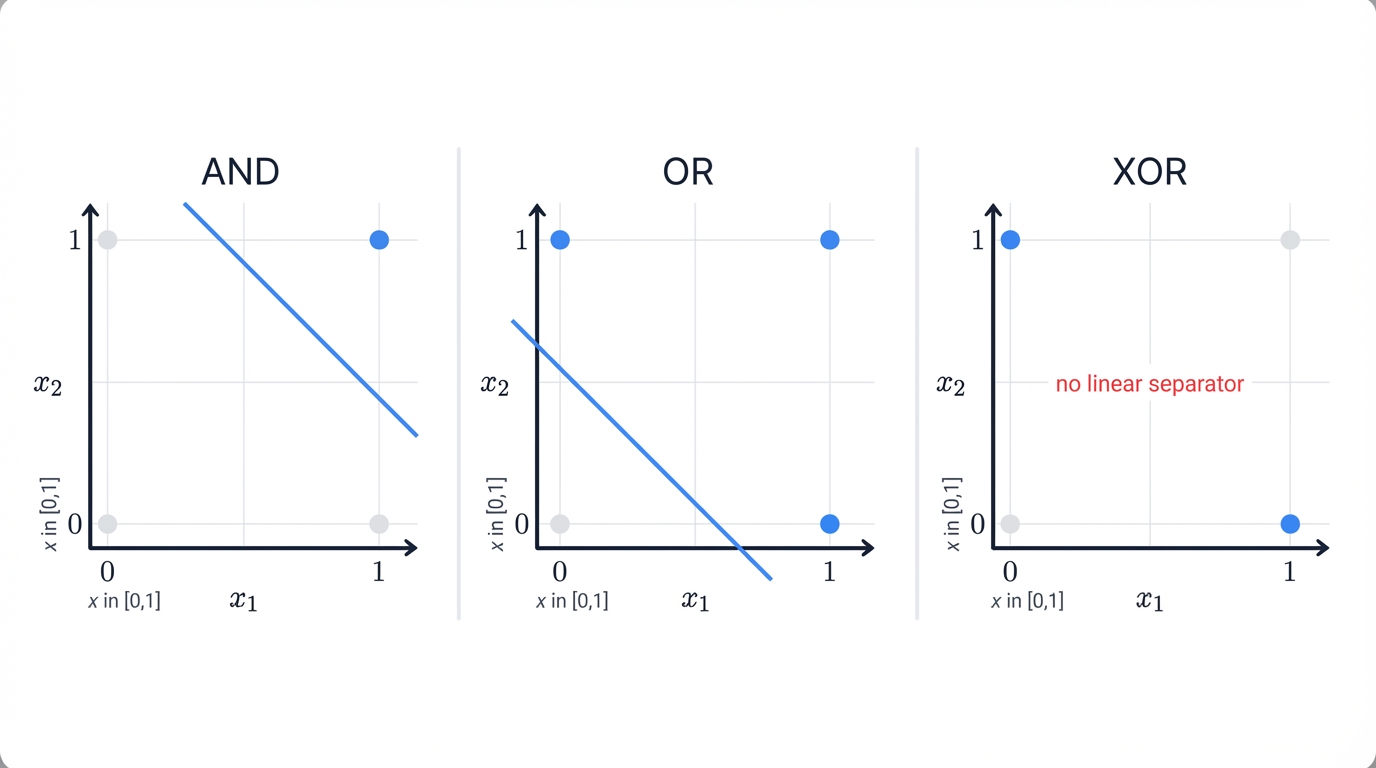
Plot these on a 2D plane. Notice something? The point (1,1) separates clearly from the other three points by a straight line. Linearly separable. Solvable by a single-layer Perceptron.
The table below walks through the Perceptron learning algorithm step-by-step as it learns to model the AND gate.
| Epoch | Input (x₁,x₂) | True Output (y) | Initial Weights (w₁,w₂,b) | Weighted Sum (z) | Predicted Output (ŷ) | Error (y-ŷ) | Weight Updates (Δw₁,Δw₂,Δb) | Final Weights (w₁,w₂,b) |
|---|---|---|---|---|---|---|---|---|
| 1 | (0, 0) | 0 | (0.3, -0.2, 0.1) | 0.1 | 1 | -1 | (0.0, 0.0, -0.1) | (0.3, -0.2, 0.0) |
| 1 | (0, 1) | 0 | (0.3, -0.2, 0.0) | -0.2 | 0 | 0 | (0.0, 0.0, 0.0) | (0.3, -0.2, 0.0) |
| 1 | (1, 0) | 0 | (0.3, -0.2, 0.0) | 0.3 | 1 | -1 | (-0.1, 0.0, -0.1) | (0.2, -0.2, -0.1) |
| 1 | (1, 1) | 1 | (0.2, -0.2, -0.1) | -0.1 | 0 | 1 | (0.1, 0.1, 0.1) | (0.3, -0.1, 0.0) |
| 2 | (0, 0) | 0 | (0.3, -0.1, 0.0) | 0.0 | 1 | -1 | (0.0, 0.0, -0.1) | (0.3, -0.1, -0.1) |
| ... | ... | ... | ... | ... | ... | ... | ... | ... |
| N | (0, 0) | 0 | (0.2, 0.2, -0.3) | -0.3 | 0 | 0 | (0.0, 0.0, 0.0) | (0.2, 0.2, -0.3) |
| N | (0, 1) | 0 | (0.2, 0.2, -0.3) | -0.1 | 0 | 0 | (0.0, 0.0, 0.0) | (0.2, 0.2, -0.3) |
| N | (1, 0) | 0 | (0.2, 0.2, -0.3) | -0.1 | 0 | 0 | (0.0, 0.0, 0.0) | (0.2, 0.2, -0.3) |
| N | (1, 1) | 1 | (0.2, 0.2, -0.3) | 0.1 | 1 | 0 | (0.0, 0.0, 0.0) | (0.2, 0.2, -0.3) |
Note: Initial weights are set randomly to w₁ = 0.3, w₂ = -0.2, b = 0.1. The learning rate η is set to 0.1. The activation function outputs 1 if z ≥ 0 and 0 otherwise. The table shows the first few updates and a final converged state where all predictions are correct.
4.2 The OR Gate (Linearly Separable)
The logical OR gate returns 1 if at least one input is 1. Truth table: (0,0) → 0, (0,1) → 1, (1,0) → 1, and (1,1) → 1.
Like the AND gate, this problem is linearly separable. The point (0,0) separates from the other three with a single line. A Perceptron learns this function easily using the same iterative weight-update process.
4.3 The XOR Problem (Non-Linearly Separable)
Here's where everything breaks down. The Exclusive OR (XOR) gate is the canonical example of Perceptron limitations.
XOR returns 1 only if its two inputs differ: (0,0) → 0, (0,1) → 1, (1,0) → 1, (1,1) → 0.
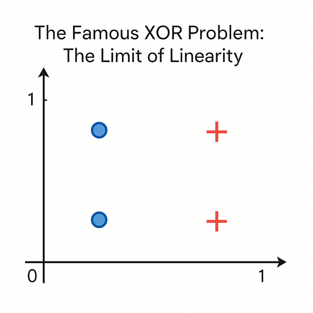
Plot these four points. Notice the pattern? Classes form a diagonal arrangement that no single straight line can separate. Points classified as '1' ((0,1) and (1,0)) sit diagonally opposite. So do points classified as '0' ((0,0) and (1,1)).
No matter where you draw a line, it misclassifies at least one point. Because the Perceptron is fundamentally a linear classifier, solving the XOR problem is mathematically impossible. When you apply the Perceptron learning algorithm to XOR data, it never converges. Weights keep adjusting indefinitely in a futile search for a non-existent linear solution.
This simple, clear failure became a powerful symbol of early neural network limits.
The Perceptron's XOR struggle wasn't a one-time mistake. It revealed a fundamental challenge that neural network research had to confront head-on, documented in an influential 1969 book that significantly reshaped how researchers viewed and approached neural networks.
5.1 Defining Linear Separability
The logic gates demonstrated the geometric property that limits single-layer Perceptron power: linear separability. Here's the formal definition: two sets of data points in n-dimensional space are linearly separable if a single hyperplane of (n-1) dimensions can divide the space such that all points from the first set lie on one side and all points from the second set lie on the other.
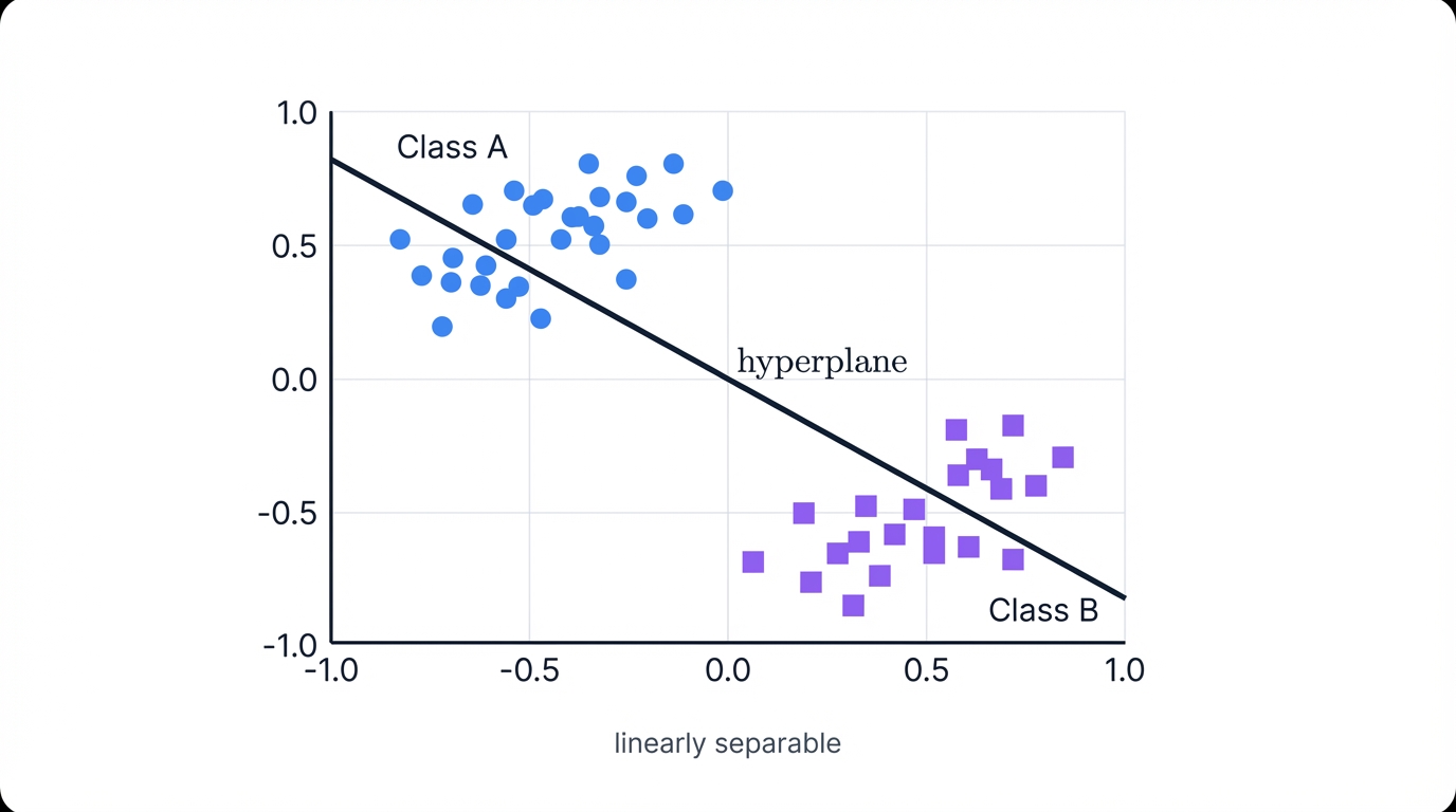
In two dimensions, this hyperplane is a line. In three dimensions, a plane. The Perceptron's architecture, based on linear combinations of inputs, makes it fundamentally a linear classifier. The learning algorithm's sole goal? Find the weights defining such a separating hyperplane.
If no such hyperplane exists, the algorithm cannot succeed. Period.
5.2 Minsky and Papert's "Perceptrons" (1969)
In 1969, MIT professors Marvin Minsky and Seymour Papert—friends and scientific critics of Rosenblatt—published Perceptrons. The book delivered a thorough, critical mathematical analysis of single-layer Perceptron computational limits.
It extended beyond the well-known XOR problem. Minsky and Papert demonstrated that Perceptrons couldn't learn certain fundamental properties of input patterns. Notable examples: parity and connectedness.
Parity? Determining whether the number of activated cells in the input "retina" is odd or even. Connectedness? Deciding if a pattern of pixels forms a single, continuous shape or breaks into multiple pieces.
They showed that solving these problems with a Perceptron would require an exponential number of connections or impossibly large weights—computationally infeasible for anything but the simplest inputs. Their main point struck hard: Perceptrons are inherently "local" machines, capable only of simple feature detection, unable to reason about "global" properties of inputs without exponential complexity increases.
This analysis wasn't just an attack. It was scientific clarification, replacing romantic, brain-inspired rhetoric with rigorous mathematical analysis. It forced the field to face the true computational limitations of its models.
5.3 The "AI Winter"
The publication of Perceptrons catalyzed the first "AI Winter"—a period from the early 1970s to mid-1980s characterized by dramatic reductions in funding and academic interest in neural network research. The book's pessimistic conclusions gave funding agencies powerful scientific justification to divert resources away from connectionist research toward other approaches like symbolic systems.
But a more nuanced historical view reveals the book as catalyst rather than sole cause. The field already faced a credibility crisis. Immense, unfulfilled hype had created a vast gap between public expectations and technical reality. Researchers had hit a genuine scientific wall: they understood single-layer network limitations but lacked viable methods for training more powerful, multi-layered networks.
Minsky and Papert's critique was the formal, mathematical nail in the coffin for research already stagnating. This perfect storm—unmanaged expectations, devastating theoretical critique, and lack of clear next steps—created a funding drought that nearly extinguished the field for over a decade.
The "AI Winter" didn't kill the Perceptron's core ideas. Instead, its well-defined failures highlighted challenges that inspired the next generation of researchers, and over time, solutions to Perceptron limitations proved its value and established its role as the foundation of modern deep learning.
6.1 The Solution: The Multi-Layer Perceptron (MLP)
The breakthrough? Adding one or more hidden layers of neurons between input and output layers, creating the Multi-Layer Perceptron (MLP).
In an MLP, each neuron in hidden layers performs basic computation similar to a single Perceptron: calculating a weighted sum of inputs, then applying a non-linear activation function. But by stacking these transformations across multiple layers, the network gains the ability to learn very complex, non-linear decision boundaries.
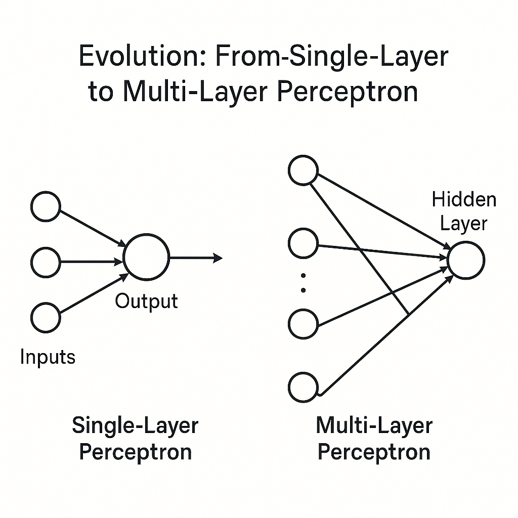
Think of the first hidden layer drawing multiple simple straight-line boundaries. Subsequent layers combine these lines to form intricate shapes—curved or enclosed regions—in feature space. This layered, hierarchical approach to learning features enables an MLP to solve non-linearly separable problems like XOR.
For example, a two-layer network transforms input space into a new, linearly separable form within its hidden layer, making output layer classification much easier.
The table below summarizes critical differences between single-layer and multi-layer architectures.
| Feature | Single-Layer Perceptron (SLP) | Multi-Layer Perceptron (MLP) |
|---|---|---|
| Architecture | Input and Output layers only. No hidden layers. | Input, one or more Hidden Layers, and Output layer. |
| Decision Boundary | Strictly Linear (a single hyperplane). | Can learn complex, Non-Linear decision boundaries. |
| Solvable Problems | Only linearly separable problems (e.g., AND, OR). | Both linearly and non-linearly separable problems (e.g., XOR, image recognition). |
| Key Limitation | Mathematically incapable of solving non-linear problems. | Prone to issues like vanishing gradients; requires more data and computational power. |
| Training Algorithm | Perceptron Learning Rule. | Backpropagation. |
6.2 From Perceptron Rule to Backpropagation
The simple Perceptron learning rule can't train a Multi-Layer Perceptron effectively. One main challenge? Figuring out how to attribute errors to weights in hidden layers, since these layers don't connect directly to final output.
A breakthrough revitalized neural network research: rediscovery and popularization of the backpropagation algorithm in the 1980s.
Backpropagation leverages the chain rule from calculus to efficiently compute how loss changes with respect to each weight in the network. It calculates error at the output layer, then carefully propagates this error backward through the network, allowing hidden neuron weights to adjust based on their contribution to overall error.
Interestingly, Rosenblatt described a similar "error correction propagation" idea in his 1962 book—a fascinating piece of history that almost predicted backpropagation, though it wasn't developed into a full algorithm at that time.
6.3 The Perceptron as the Foundational Unit of Deep Learning
The Perceptron's impact is both significant and paradoxical. Its straightforward single-layer design had clear limitations that spurred further AI innovations. Its shortcomings motivated researchers to explore complex, multi-layer structures and led to backpropagation algorithm development, which became a cornerstone of modern neural networks.
However, core Perceptron ideas have proven remarkably enduring. The basic concept of an artificial neuron—a unit that takes inputs, computes a weighted sum, adds a bias, and applies non-linear activation—remains fundamental today.
Whether in the latest Transformer models or Convolutional Neural Networks, neurons perform essentially the same mathematical operation Rosenblatt introduced in 1957. Activation functions evolved from step functions to smoother options like Sigmoid and ReLU. Learning algorithms advanced from the original Perceptron rule to powerful backpropagation combined with modern optimizers.
Despite these developments, the humble Perceptron remains the foundational building block, the "atom" that continues to underpin the vast, complex world of deep learning.
Conclusion: The First Stepping Stone
Best Practice: Following these recommended practices will help you achieve optimal results and avoid common pitfalls.
The Perceptron story? Fascinating. Revolutionary. Cautionary. It began as an innovative idea inspired by biological learning, suggesting machines could learn from experience too. Initial excitement ran high. But as time passed, serious limitations emerged, leading to the "AI Winter"—a period when funding and interest in AI plummeted, partly due to strict mathematical critiques exposing the gap between hype and reality.
But the story didn't end there. The lessons learned from these challenges paved the way for the next big leap: the Multi-Layer Perceptron. With backpropagation algorithm introduction, this new model handled complex, non-linear problems the original Perceptron couldn't solve.
Today? You won't find single-layer Perceptrons in everyday applications. Their true value lies in what they taught us—the first real step toward modern AI. The Perceptron established fundamental connectionist AI ideas and, through successes and failures, laid groundwork for the entire neural network revolution.
For anyone curious about deep learning history, theory, or core principles, exploring the Perceptron story is where the journey begins.
Key Takeaways:
- The Perceptron introduced machine learning through adaptive weights
- Its linear architecture limits it to linearly separable problems
- The XOR problem demonstrated fundamental limitations that led to the AI Winter
- Multi-layer architectures and backpropagation overcame these limitations
- The basic neuron concept remains central to modern deep learning systems