Every neural network learns through the same fundamental cycle. Data flows forward through the network. The model makes a prediction. You compare that prediction to the actual answer and calculate how wrong it was. Then you work backwards through the network, computing gradients that tell you how to adjust each weight. Finally, you update those weights to reduce the error.
This guide breaks down that cycle into its essential components. You'll learn what tensors are, how weights transform data, which activation functions introduce non-linearity, and how optimizers adjust parameters. Each section provides formulas, code examples, and practical context.
High-Level Flow: Application to Output
Pipeline: Input Data → Preprocessing → Model (Neural Network) → Output → Loss Calculation → Backpropagation → Weight Update → Repeat
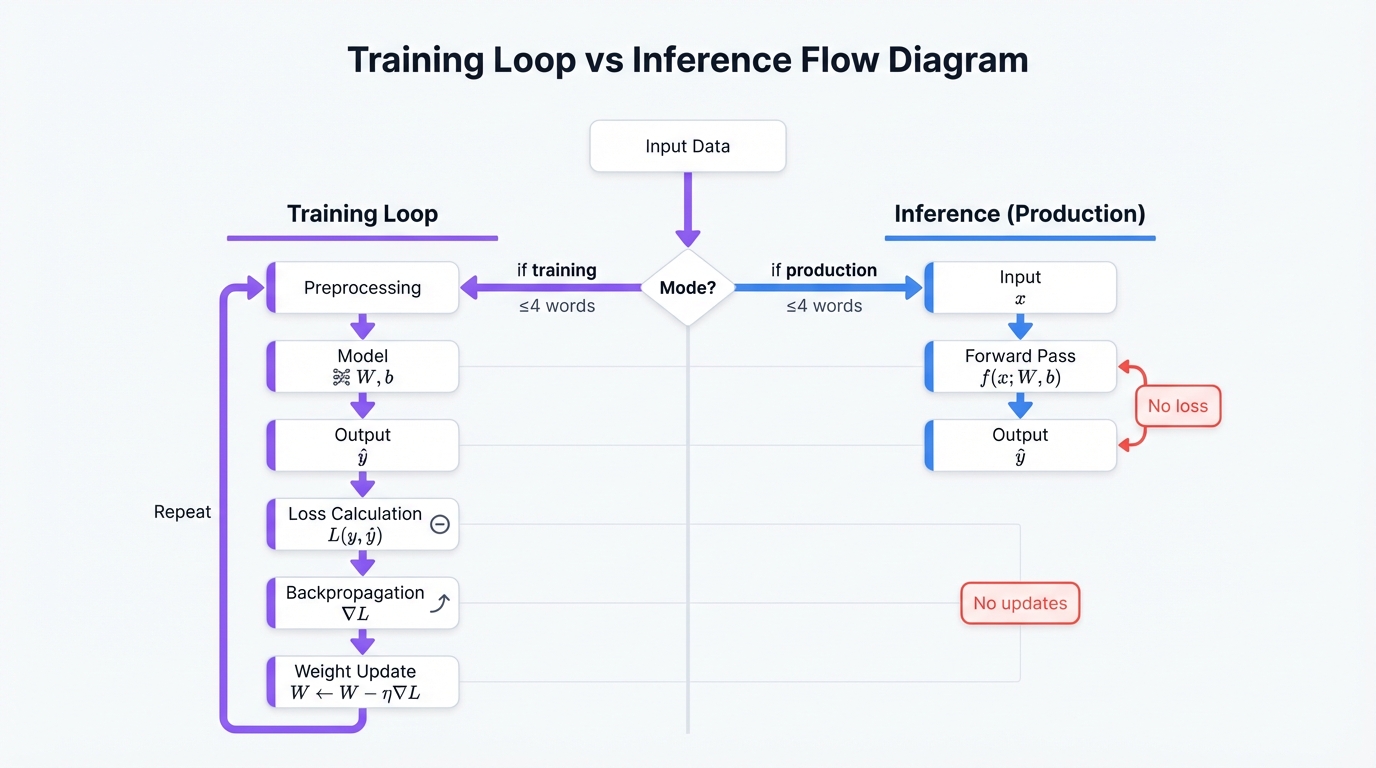
Training Loop
Every neural network learns through the same fundamental cycle. Data flows forward through the network. The model makes a prediction. You compare that prediction to the actual answer and calculate how wrong it was. Then you work backwards through the network, computing gradients that tell you how to adjust each weight. Finally, you update those weights to reduce the error.
Here's the step-by-step breakdown:
- Forward Pass: Data flows through layers and produces a prediction.
- Loss Calculation: Compare the prediction to the actual answer.
- Backward Pass: Compute gradients showing how to adjust weights.
- Optimization: Update weights to reduce error.
- Repeat: Move to the next batch of data.
Inference (Production)
When your model goes into production, the process simplifies dramatically. You run only the forward pass. Input data enters the network, flows through the trained layers, and produces an output. That's it.
No loss calculation happens. No weight updates occur. The model uses the knowledge it learned during training to make predictions on new data.
The production flow: Input → Forward Pass → Output
Tensors
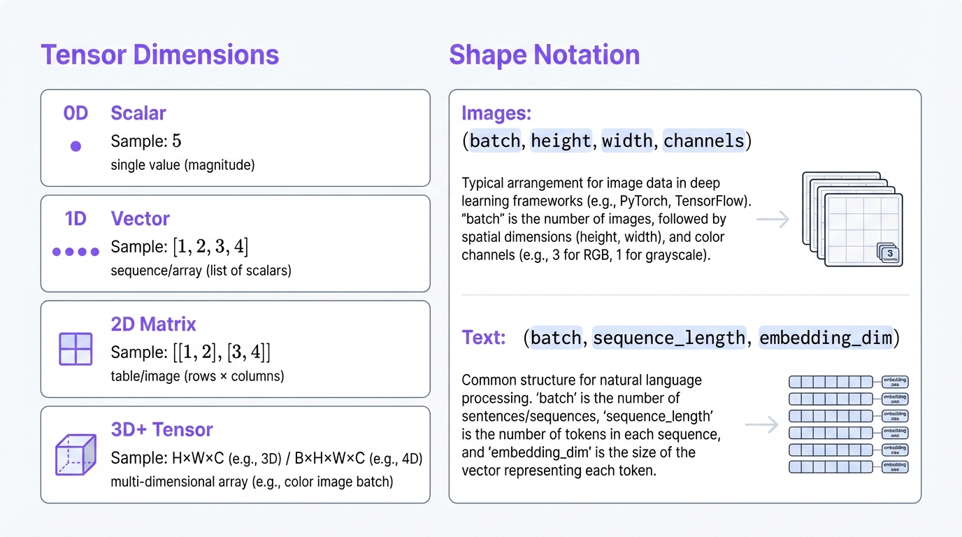
What they are: Multi-dimensional arrays of numbers. Think of tensors as containers that hold your data in a structure the neural network can process.
Dimensions
Tensors come in different shapes depending on what kind of data you're working with:
- 0D (Scalar): A single number →
5 - 1D (Vector): An array of numbers →
[1, 2, 3, 4] - 2D (Matrix): A table of numbers →
[[1, 2], [3, 4]] - 3D+: Higher dimensions for complex data → images are height × width × channels
Shape Notation
The shape tells you the dimensions of your tensor. Different types of data use different shape conventions:
- Images:
(batch_size, height, width, channels) - Text:
(batch_size, sequence_length, embedding_dim)
Batch size always comes first. It represents how many examples you're processing simultaneously.
Example
Here's what a batch of images looks like:
# Batch of 32 images, 224x224 pixels, 3 color channels (RGB)
image_tensor.shape  # → (32, 224, 224, 3)
This tensor holds 32 RGB images, each 224 pixels tall and 224 pixels wide. The 3 represents the red, green, and blue color channels.
Weights (Parameters)
What they are: Learnable numbers that transform inputs into outputs.
What they do: Store the knowledge your network learns during training.
Types
Neural networks use two types of parameters:
Weight matrices connect neurons between layers. They determine how strongly each input influences each output. During training, the network adjusts these weights to recognize patterns in your data.
Biases shift activation values, similar to the y-intercept in linear equations. They give the network additional flexibility to fit complex patterns.
Example
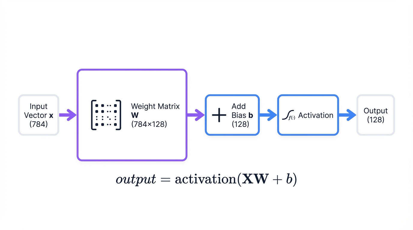
Consider a dense layer that transforms 784 input features into 128 output features:
# Dense layer: input_size=784, output_size=128
weights.shape  # → (784, 128)   # Transform 784 features to 128
bias.shape     # → (128,)       # One bias per output neuron
At the start of training, weights initialize randomly. As training progresses, the optimizer adjusts them to minimize the loss function. By the end, these weights encode the patterns your network learned.
Layers
What they are: Building blocks that transform data as it flows through your network.
Each layer type serves a specific purpose. Some detect visual patterns. Others process sequences or reduce dimensions. Understanding when to use each type is crucial for building effective models.
Common Layer Types
Dense (Fully Connected)
Every input neuron connects to every output neuron. The layer computes output = activation(input × weights + bias). Use dense layers for final classification stages where you need to combine all learned features.
Convolutional (Conv2D)
These layers scan images with small filters, detecting patterns like edges, textures, and objects. Convolutional layers excel at image processing because they preserve spatial relationships between pixels.
Recurrent (LSTM, GRU)
Recurrent layers maintain memory of previous inputs, making them ideal for sequential data. Use them for text analysis, time series prediction, or any task where context from earlier inputs matters.
Pooling
Pooling layers reduce spatial dimensions by summarizing regions. Max pooling takes the maximum value in each region. Use pooling between convolutional layers to progressively downsample feature maps.
Dropout
During training, dropout randomly zeros out neurons. This prevents the network from relying too heavily on any single neuron, reducing overfitting. The network learns more robust features that generalize better to new data.
Batch Normalization
Batch normalization normalizes inputs to each layer, stabilizing and accelerating training. It reduces internal covariate shift, allowing you to use higher learning rates and train deeper networks successfully.
Activations (Activation Functions)
What they are: Non-linear functions applied after layer computations.
Why they matter: Without activations, stacking multiple layers would be pointless. The network would collapse into a simple linear model, no matter how many layers you added.
Activations introduce non-linearity. They let networks learn complex patterns and make sophisticated decisions.
Common Activations
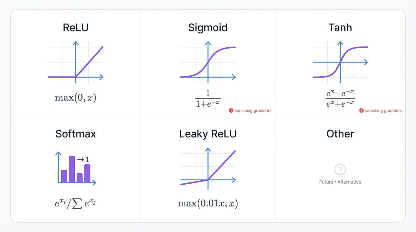
ReLU (Rectified Linear Unit)
Formula: f(x) = max(0, x)
ReLU is the most common activation. It's fast, simple, and effective. The function outputs zero for negative inputs and passes positive values unchanged.
One weakness: neurons can die if their inputs stay negative throughout training. The gradient becomes zero, and the neuron stops learning.
Sigmoid
Formula: f(x) = 1 / (1 + e-x)
Sigmoid squashes inputs into the range [0, 1]. Use it for binary classification outputs where you need a probability. Avoid it in hidden layers—the gradients can vanish, making deep networks hard to train.
Tanh
Formula: f(x) = (ex - e-x) / (ex + e-x)
Tanh outputs values in [-1, 1]. It's zero-centered, which often makes it work better than sigmoid for hidden layers. But it still suffers from vanishing gradients in very deep networks.
Softmax
Formula: f(xi) = exi / Σj exj
Softmax converts raw scores (logits) into probabilities that sum to 1. Use it as the final activation for multi-class classification. It tells you the network's confidence for each possible class.
Leaky ReLU
Formula: f(x) = max(0.01x, x)
Leaky ReLU fixes the dying neuron problem. Instead of outputting zero for negative inputs, it passes a small gradient (typically 0.01). This keeps neurons learning even when their inputs are negative.
Loss Functions
What they are: Measures of how wrong your predictions are.
Your goal: Minimize loss during training.
The loss function quantifies the gap between predictions and reality. It gives the optimizer a target to optimize. Choose the wrong loss function, and your network won't learn what you want it to learn.
Common Losses
Mean Squared Error (MSE)
Formula: MSE = (1/n) Σ (ŷ - y)²
MSE calculates the average squared difference between predictions and actual values. Use it for regression problems where you're predicting continuous values, like house prices or temperatures.
Binary Cross-Entropy
Formula: L = -[y log p + (1-y) log(1-p)]
Binary cross-entropy measures the difference between two probability distributions for binary outcomes. Use it for binary classification tasks like spam detection or fraud identification.
Categorical Cross-Entropy
Formula: L = -Σi yi log pi
Categorical cross-entropy extends binary cross-entropy to multiple classes. Use it when each example belongs to exactly one category, like ImageNet classification with 1,000 possible objects.
Sparse Categorical Cross-Entropy
This works like categorical cross-entropy but accepts integer labels instead of one-hot encoded vectors. It's more memory-efficient for problems with many classes.
Optimization (Optimizers)
What they are: Algorithms that adjust weights to minimize loss.
Core concept: Gradient descent—move weights in the direction that reduces loss.
Optimizers determine how your network learns. They take the gradients from backpropagation and use them to update weights. Different optimizers make different tradeoffs between speed, stability, and memory usage.
Common Optimizers
SGD (Stochastic Gradient Descent)
Formula: weight = weight - learning_rate × gradient
SGD is the simplest optimizer. It updates weights directly based on the gradient. Simple and reliable, but it can get stuck in local minima. Typical learning rates range from 0.01 to 0.1.
Adam (Adaptive Moment Estimation)
Adam adapts the learning rate for each parameter individually. It's the most popular optimizer because it works well across a wide range of problems with minimal tuning. Start with a learning rate of 0.001.
RMSprop
RMSprop adapts learning rates based on recent gradients. It works particularly well for recurrent neural networks, where gradient scales can vary dramatically across time steps.
SGD with Momentum
Momentum adds velocity along consistent gradient directions. Instead of taking small steps based only on the current gradient, the optimizer builds momentum, helping it escape local minima and converge faster.
Hyperparameters
Learning Rate (LR)
Controls how much to adjust weights each step.
Set it too high and training becomes unstable or diverges completely. Set it too low and training crawls along, potentially getting stuck in poor local minima. Typical values range from 0.001 to 0.01.
Batch Size
Determines how many samples you process before updating weights.
Small batches (32 examples) create noisy gradients with a regularization effect. Large batches (256 examples) produce stable gradients and faster training per epoch. Typical values: 32, 64, or 128.
Softmax (Detailed)
What it is: A function that converts raw scores (logits) to probabilities.
Formula: softmax(xi) = exi / Σj exj
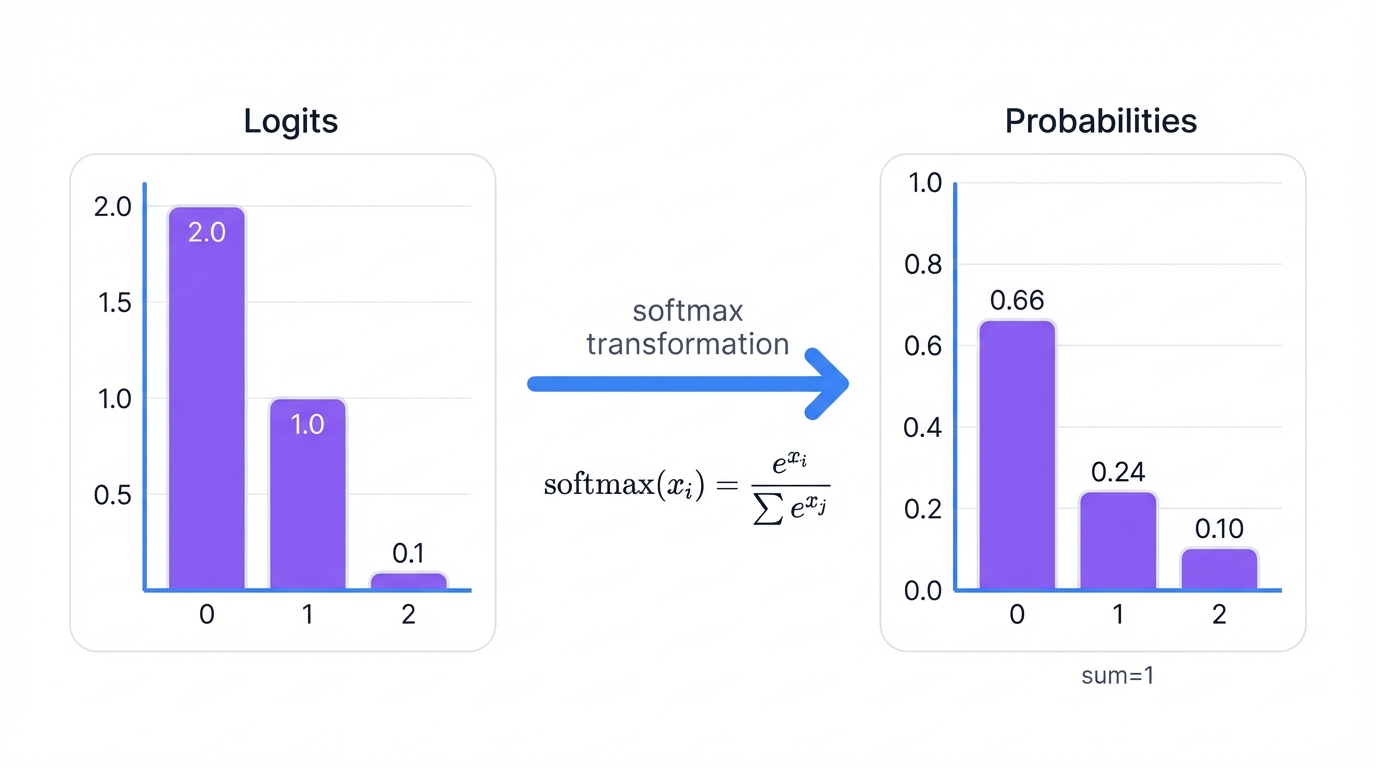
Softmax takes a vector of arbitrary real numbers and transforms them into a valid probability distribution. The outputs are all positive and sum to exactly 1.
Example
Watch how softmax transforms raw model outputs:
# Raw model output (logits)
logits = [2.0, 1.0, 0.1]

# After softmax
probabilities = [0.659, 0.242, 0.099]  # Sum = 1.0

# Interpretation
# Class 0: 65.9% confidence
# Class 1: 24.2% confidence
# Class 2: 9.9% confidence
The network is most confident about class 0, moderately confident about class 1, and least confident about class 2.
Use Cases
Multi-class classification: Softmax appears in the final layer of classifiers that choose between multiple categories.
Attention mechanisms: Transformers use softmax to compute attention weights, determining which parts of the input to focus on.
Policy networks: Reinforcement learning agents use softmax to convert action values into action probabilities.
Why Exponential?
The exponential function serves three critical purposes:
It amplifies differences between logits, making the probability distribution sharper. It ensures all outputs are positive, which is required for valid probabilities. And it produces a valid probability distribution where all values sum to 1.
Complete Example: Image Classification
Here's how all the pieces fit together in a real image classification network:
# 1) INPUT: Batch of 32 cat/dog images
input_tensor.shape  # → (32, 224, 224, 3)  # RGB images

# 2) LAYERS (Forward Pass)
conv1_output   = Conv2D(32, ...)(input_tensor)   # Extract features
pool1_output   = MaxPool2D(...)(conv1_output)    # Downsample
conv2_output   = Conv2D(64, ...)(pool1_output)   # More features
pool2_output   = MaxPool2D(...)(conv2_output)    # Downsample
flatten_output = Flatten()(pool2_output)         # 2D → 1D
dense1_output  = Dense(128, activation='relu')(flatten_output)  # Classification head
logits         = Dense(2)(dense1_output)         # 2 classes (cat/dog)

# 3) ACTIVATION (Softmax)
probabilities = softmax(logits)
# Example: [0.85, 0.15] → 85% dog, 15% cat

# 4) LOSS (During Training)
true_label = [1, 0]  # Dog = class 0
loss = categorical_crossentropy(true_label, probabilities)

# 5) OPTIMIZATION (Backpropagation)
gradients = compute_gradients(loss)
optimizer.apply_gradients(gradients)  # Update all weights

# 6) REPEAT with next batch
The first convolutional layer detects simple features like edges and corners. Pooling reduces the spatial dimensions. The second convolutional layer combines those simple features into more complex patterns like textures and shapes.
After flattening, the dense layer acts as a classifier. It looks at all the detected features and decides whether the image shows a cat or dog. Softmax converts the raw scores into probabilities.
During training, the loss function measures how wrong the prediction was. Backpropagation computes gradients, and the optimizer updates weights. The network repeats this process thousands of times, gradually improving its accuracy.
Key Formulas
Dense Layer
output = activation(XW + b)
This is the fundamental operation of a fully connected layer. Multiply inputs by weights, add bias, and apply an activation function.
Gradient Descent
wnew = wold - η · ∂L/∂w
Update each weight by subtracting the learning rate (η) multiplied by the gradient of the loss with respect to that weight.
Batch Normalization
output = γ · (x - μ) / σ + β
Normalize inputs by subtracting the mean (μ) and dividing by standard deviation (σ), then scale by γ and shift by β. Both γ and β are learnable parameters.
Dropout (Training)
output = input × binary_mask / keep_probability
Randomly zero out neurons by multiplying by a binary mask, then scale remaining activations by dividing by the keep probability. This ensures the expected value stays constant.
Common Architectures
Feedforward (MLP):
Input → Dense → ReLU → Dense → ReLU → Dense → Softmax
The simplest architecture. Data flows forward through fully connected layers. Each layer learns increasingly abstract representations.
CNN (Image):
Input → Conv → ReLU → Pool → Conv → ReLU → Pool → Flatten → Dense → Softmax
Convolutional networks extract spatial features from images. Early layers detect edges and textures. Later layers recognize objects and scenes.
RNN (Sequence):
Input → Embedding → LSTM → LSTM → Dense → Softmax
Recurrent networks process sequences, maintaining hidden state across time steps. They excel at tasks where context and order matter.
Transformer (Modern NLP):
Input → Embedding → Multi-Head Attention → FFN → Layer Norm → (Repeat × N) → Dense
Transformers use attention mechanisms instead of recurrence. They process entire sequences in parallel, making them faster to train and better at capturing long-range dependencies.
Training vs Inference
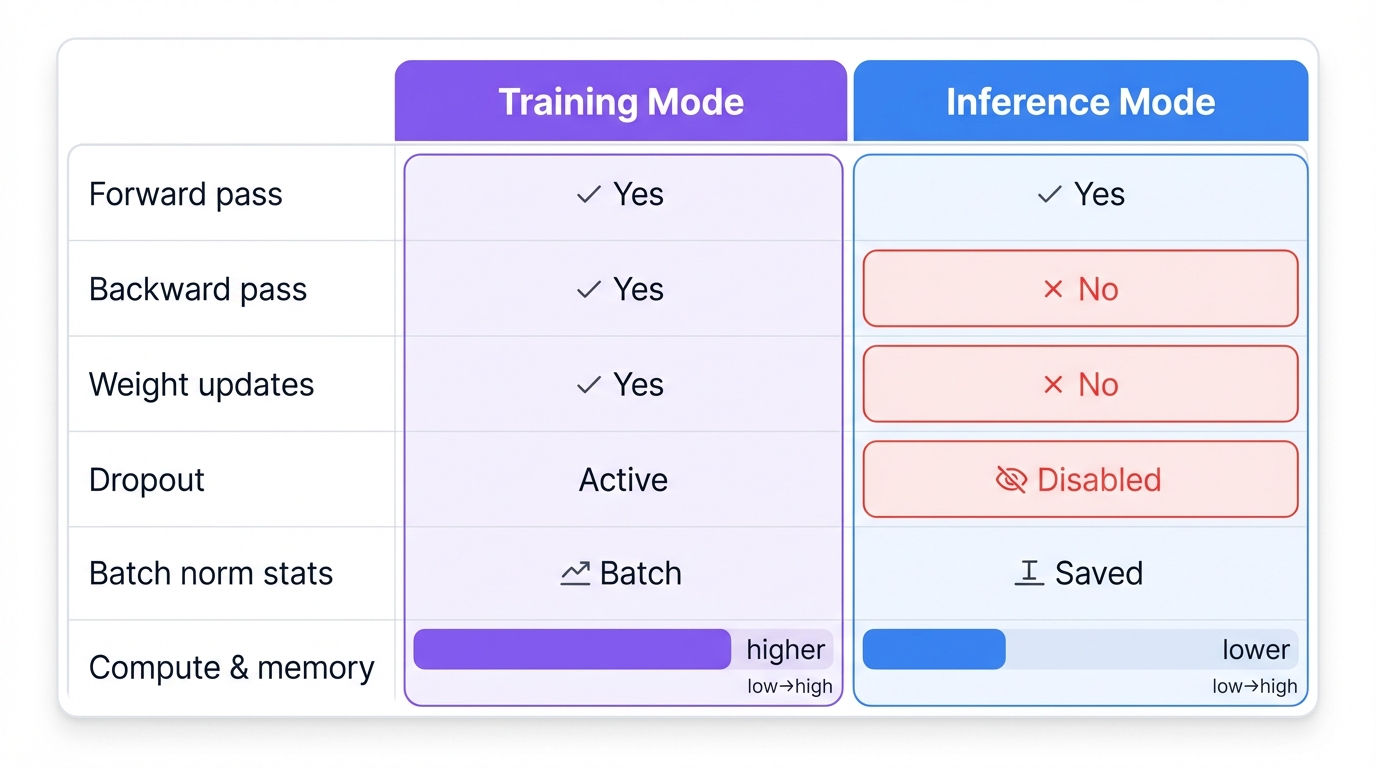
Training Mode
During training, your network learns from data. The forward pass calculates predictions. The backward pass calculates gradients showing how to improve. Weight updates adjust parameters to reduce loss.
Dropout is active—neurons randomly drop out to prevent overfitting.
Batch normalization updates running statistics based on the current batch.
Training requires significantly more computation and memory than inference.
Inference Mode
In production, the network uses its learned knowledge to make predictions on new data. Only the forward pass runs. Weights stay frozen—no updates occur.
Dropout is disabled—all neurons remain active for consistent predictions.
Batch normalization uses saved statistics from training, not the current batch.
Inference is faster and requires less memory than training.
Quick Reference
| Concept | Purpose | Example |
|---|---|---|
| Tensor | Data container | Image: (32, 224, 224, 3) |
| Weight | Learnable parameter | Dense layer: (784, 128) |
| Bias | Shift activation | One per neuron |
| Layer | Data transformation | Conv2D, Dense, LSTM |
| Activation | Non-linearity | ReLU, Softmax |
| Loss | Error measurement | Cross-entropy |
| Optimizer | Weight updater | Adam |
| Batch Size | Samples per update | 32, 64, 128 |
| Learning Rate | Update step size | 0.001, 0.01 |
| Epoch | Full dataset pass | 100 epochs |
Conclusion
Neural networks combine simple mathematical operations—matrix multiplication, addition, activation functions—into powerful learning systems. You now understand how tensors hold data, how weights transform inputs, how layers build hierarchical representations, and how optimizers adjust parameters to minimize loss.
The training loop is straightforward: forward pass generates predictions, loss calculation measures error, backward pass computes gradients, and optimization updates weights. In production, you run only the forward pass with frozen weights.
Use this guide as a reference when building neural networks. Refer back to the layer types when choosing architectures. Check the activation functions when deciding how to introduce non-linearity. Review the optimizer section when tuning hyperparameters. The fundamentals don't change—only the scale and complexity.
What's Next?
Continue your learning journey with these related articles: