Table of Contents
Magic? No. Your machine learning models are mathematical engines.
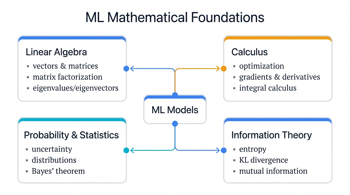
When your recommendation system suggests the perfect product or your fraud detection flags a suspicious transaction, intuition isn't at work. Mathematics is. Four mathematical domains power every ML algorithm you'll ever encounter: Linear Algebra, Calculus, Probability & Statistics, and Information Theory.
Here's what matters. Understanding these foundations isn't an academic luxury—it's a practical necessity for anyone building systems that actually work in production.
Think about it. When attackers exploit your models through adversarial examples, they weaponize the same math that makes your systems work. When your models fail in production, the root cause lives in these mathematical principles. When training mysteriously stalls at 3 AM, the answer hides in the mathematics, waiting for you to discover it and fix the problem before your stakeholders wake up.
We'll explore each domain with real-world examples, then show you exactly how cybercriminals exploit these same foundations in Adversarial Machine Learning attacks.
Why Linear Algebra Runs Your Business (Whether You Know It or Not)
Netflix processes 2 billion hours of viewing data monthly. Amazon analyzes millions of purchase patterns. Your fraud detection scans thousands of transactions per second. Every single operation relies on linear algebra.
Picture this. Netflix processes 2 billion hours of viewing data monthly to recommend your next binge. Amazon analyzes millions of purchase patterns to suggest products you didn't know you needed. Your fraud detection system scans thousands of transactions per second, catching criminals before they strike.
Every single operation? Linear algebra.
You're Already Using It
When your recommendation engine suggests products, it multiplies massive user-item matrices behind the scenes. Each customer becomes a vector of preferences—compact, mathematical, precise. Each product becomes a vector of features. Your system multiplies these vectors millions of times per second to generate recommendations that drive 35% of Netflix's viewing and 35% of Amazon's revenue.
Think about your customer data for a moment. Every row in your database is a vector carrying information about behavior, preferences, and potential. Every feature—age, purchase history, location—becomes a column in your data matrix. When you train models to predict customer behavior, you're essentially solving giant systems of linear equations that would make your college math professor proud. Your model parameters? They're matrices. Your predictions? Matrix-vector multiplications happening at speeds humans can barely comprehend.
Here's the business impact that executives actually care about: Companies that optimize their linear algebra operations see 10-100x speed improvements in model training and inference, and that performance boost translates directly to faster time-to-market and dramatically lower infrastructure costs that make CFOs smile.
The Breakthrough Moment: When Linear Algebra Saves Your Project
You're three weeks into your customer churn prediction project. Your data scientist just handed you a model that needs to process 10 million customer records to predict who's likely to cancel. Without optimization, it takes 6 hours—an eternity in business time. Your business needs real-time predictions.
Enter linear algebra optimization.
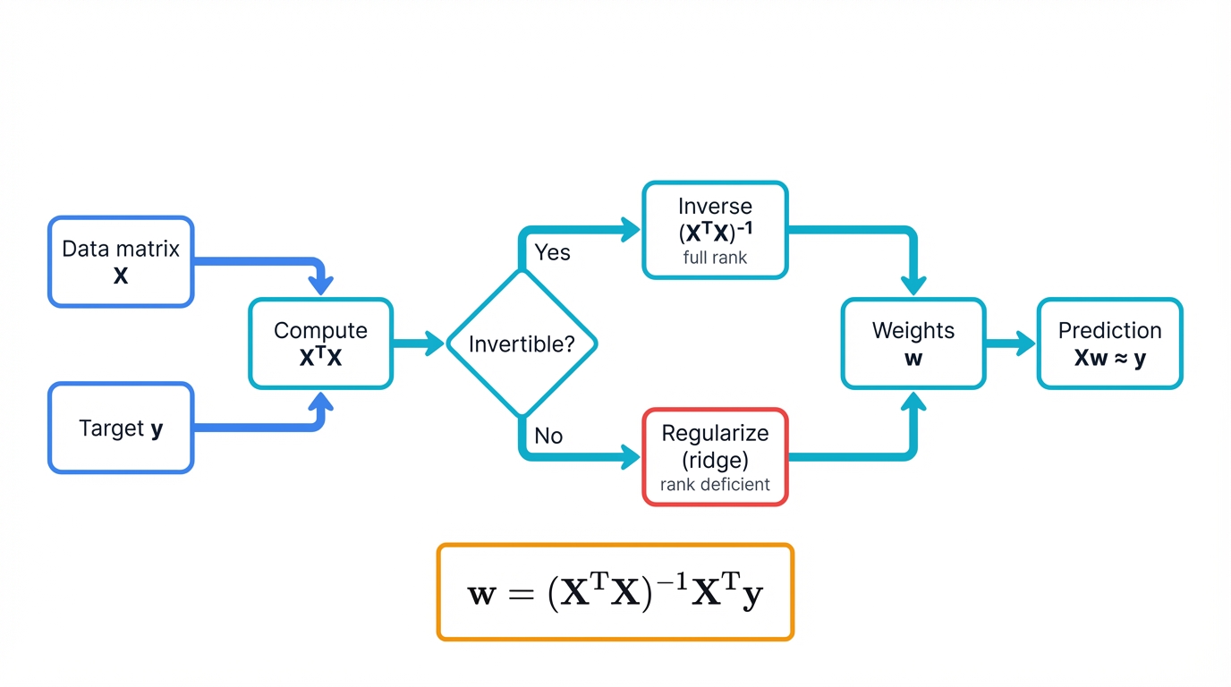
Your linear regression model becomes an elegant equation: $Xw \approx y$. Simple. Beautiful. Here, $X$ holds your customer data matrix, $w$ contains the weights that determine importance of each feature, and $y$ represents your target outcomes. The Normal Equation $w = (X^T X)^{-1} X^T y$ solves this in one shot using matrix operations that computers handle with breathtaking efficiency.
The business impact? Your 6-hour processing time drops to 6 minutes—a 60x improvement that changes everything about how you operate. You can now run predictions hourly instead of daily. Customer retention campaigns become proactive instead of reactive. You catch problems before they become losses.
Matrix transposes—flipping rows and columns—and matrix inverses become your computational workhorses doing the heavy lifting. When the inverse exists, you get a unique solution. When it doesn't, you discover your data has fundamental issues that need addressing before any model will work reliably.
Matrix Rank: Why Your Model Sometimes Refuses to Learn
You've built a customer segmentation model with 50 features. Training keeps failing with cryptic "singular matrix" errors. Your data looks fine. What's happening?
The problem is rank deficiency. Your feature matrix doesn't have full rank—some features are linear combinations of others, creating mathematical redundancy that breaks your algorithms like a house of cards.
Matrix rank measures the number of linearly independent rows or columns in your matrix. A matrix with $n$ columns has rank $n$ only if all columns provide unique information. When rank is less than $n$, you have redundancy—wasted computation and broken training.
Real-world causes of rank deficiency lurk in your data pipelines:
- Perfect multicollinearity occurs when one feature is an exact combination of others, such as "total_price = unit_price × quantity" creating redundant columns that confuse your model
- Duplicate features can enter your dataset through data pipeline errors, giving you the same information twice and wasting computational resources
- One-hot encoding errors happen when you keep all dummy variables instead of dropping one, introducing mathematical dependency that crashes training
- Insufficient data becomes a problem when you have more features than samples, making your matrix mathematically underdetermined and impossible to solve uniquely
The business consequence? Your model can't learn unique weights for each feature. The optimization problem becomes ill-posed—mathematically unsolvable. Training fails or produces unstable, meaningless results that waste weeks of work.
The solution: Check matrix rank before training. Remove redundant features ruthlessly. Use regularization to handle near-singular matrices. This isn't just debugging—it's fundamental data quality control that separates professionals from amateurs.
Matrix Conditioning: When Small Errors Become Big Problems
Your model trains successfully with 95% accuracy. You deploy to production. Within weeks, predictions drift wildly without warning. Small changes in input data produce massive swings in output. Your model has become unreliable.
The culprit? Poor matrix conditioning.
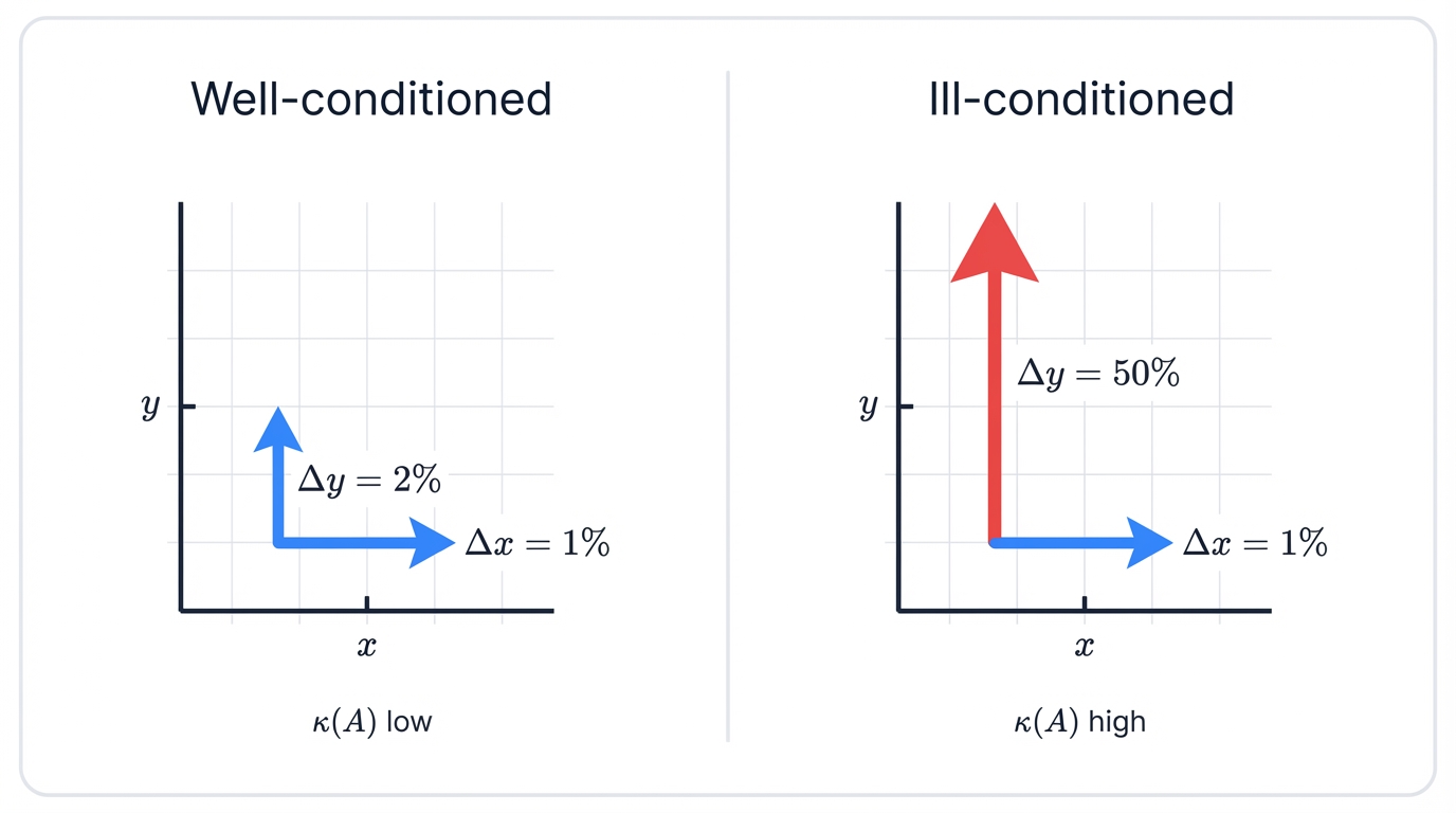
A matrix's condition number measures how sensitive its inverse is to small changes in input—think of it as the stability score for your mathematical operations. High condition numbers (≥1000) mean your matrix is "ill-conditioned"—tiny input perturbations cause huge output changes that destroy reliability.
The mathematical measure: $\kappa(A) = |A| |A^{-1}|$
When $\kappa(A)$ is large, your system becomes numerically unstable—a mathematical disaster waiting to happen. This happens when:
- Features have vastly different scales—income in dollars versus age in years—creating numerical instability during computation that compounds with each operation
- Near-collinear features provide almost duplicate information, making the matrix nearly singular and dangerously unstable
- Floating-point precision limits cause rounding errors to accumulate and compound during computation, turning small errors into catastrophic failures
Business impact cascades through your systems:
- Unstable predictions change dramatically with minor input variations, making your model unreliable for business decisions that matter
- Training becomes sensitive to initialization, producing different results each run and making reproducibility impossible
- Model coefficients grow unreasonably large, indicating mathematical instability rather than genuine feature importance
The fix requires disciplined engineering:
- Feature scaling through standardization or normalization brings all features to similar ranges, preventing scale-related instability
- Ridge regularization adds a small value to diagonal elements, improving conditioning and stabilizing solutions
- Eigenvalue analysis identifies problematic directions in your data that need correction before deployment
Professional teams always check condition numbers before deployment. It's the difference between stable production systems and models that fail mysteriously in the wild.
How Eigenvalues Cut Your Data Storage Costs by 90%
Your company just hit 50 million customer records with 500 features each. Storage costs are exploding. Training takes forever. Your models are struggling with the curse of dimensionality.
Eigenvalues and eigenvectors save the day.
Think of eigenvectors as special directions in your data where important patterns live—the mathematical highways where information flows most efficiently. When you apply a transformation (matrix) to an eigenvector $v$, it only stretches or shrinks along that same direction: $A v = \lambda v$. The eigenvalue $\lambda$ tells you how much stretching occurs—the importance of that direction.
Principal Component Analysis (PCA) finds these special directions in your customer data through mathematical elegance that borders on magic. It discovers which combinations of features contain the most information. Often, 95% of your data's important patterns live in just 10% of the dimensions—a stunning compression ratio that transforms storage economics.
Real-world result: You keep 50 features instead of 500. Storage costs drop 90%. Training time drops from days to hours. Model accuracy stays the same or improves because you've eliminated noise.
This isn't just compression—it's pattern discovery. You're identifying the fundamental patterns that drive customer behavior.
The mathematical process unfolds systematically:
- Center your data by subtracting means
- Compute the covariance matrix $C = \frac{1}{n}X^T X$
- Find eigenvalues and eigenvectors of $C$
- Keep eigenvectors with largest eigenvalues
- Project data onto these principal components
Each eigenvalue tells you how much variance that component captures—the importance score for that direction. Plot them in descending order (a "scree plot"), and you'll see how many components you actually need to capture your data's essence.
Orthogonality is PCA's secret weapon that makes everything work beautifully. The principal components are orthogonal—perpendicular to each other—meaning they capture independent patterns that don't overlap or interfere. No redundancy. No overlap. Pure, uncorrelated information flowing through independent channels.
This mathematical guarantee prevents the multicollinearity problems that plague high-dimensional data. Your new features are provably independent.
SVD: The Swiss Army Knife of Data Science
Singular Value Decomposition works where eigenvalues can't. While eigenvalues only work with square matrices, SVD handles any data matrix—tall, wide, or square—with mathematical grace and computational efficiency.
SVD breaks any matrix $A$ into three components: $U \Sigma V^T$. Think of it as finding the perfect way to represent your data using fewer pieces while keeping the important information intact.
The mathematical breakdown reveals the elegance:
- $U$ contains left singular vectors capturing patterns in rows and samples
- $\Sigma$ is a diagonal matrix of singular values showing importance weights
- $V^T$ contains right singular vectors capturing patterns in columns and features
The singular values in $\Sigma$ appear in descending order by mathematical necessity. Large values indicate important patterns worth keeping. Small values indicate noise worth discarding. Truncate the small ones, and you get lossy compression that preserves meaning while slashing storage costs.
Where you'll use SVD becomes clear when you examine real applications:
SVD enables practical applications that generate billions in business value across multiple domains:
- Netflix-style recommendations leverage SVD-powered collaborative filtering by finding hidden patterns between users and movies that enable accurate preference predictions and personalized content delivery that keeps viewers engaged
- Document analysis uses SVD variants like Latent Semantic Analysis to understand which documents relate to which topics, enabling more relevant search results and content organization that users actually find useful
- Image compression applies SVD to reduce file sizes by 10x while maintaining visual quality, enabling faster web delivery and reduced storage costs without noticeable quality loss
- Noise reduction works by dropping small singular values to eliminate noise while preserving signal integrity, improving data quality for downstream analysis and better business decisions
Your competitive advantage crystallizes here: Companies using SVD for recommender systems see 15-25% increases in conversion rates that translate directly to revenue. Document search becomes dramatically more relevant, improving user satisfaction. Image processing pipelines run faster with smaller file sizes, reducing infrastructure costs across the board.
Sparse Matrices: Scaling to Billions of Features
Your recommendation system needs to handle 10 million users and 100,000 products. That's a trillion possible user-item pairs. Storing this as a dense matrix would require 8 terabytes of RAM. Impossible.
Sparse matrices solve this elegantly by storing only non-zero values—a brilliant compression scheme that makes the impossible routine. Most users rate only a tiny fraction of products. Your trillion-element matrix might have only 100 million ratings—99.99% sparse.
Business applications demonstrate the power:
- Text processing represents documents as term-document matrices where most words don't appear in most documents, creating massive sparsity that sparse matrices handle efficiently
- Graph data stores social networks as adjacency matrices where most people aren't connected to most others—natural sparsity that sparse representations exploit
- Recommender systems handle user-item interactions where users engage with tiny fractions of available items, creating sparsity that makes storage tractable
Specialized sparse matrix operations run 1000x faster and use 1/100th the memory of dense alternatives—performance improvements that transform economics. Libraries like SciPy provide optimized implementations that make billion-parameter models practical for production deployment.
Tensors: Beyond Two Dimensions
Modern deep learning moves beyond matrices into tensors—multi-dimensional arrays that represent complex data structures with mathematical precision.
A color image is a 3D tensor: height × width × color channels. A video is a 4D tensor: time × height × width × channels. A batch of videos for training becomes a 5D tensor—complexity managed through mathematical abstraction.
Tensor operations power breakthrough applications:
- Convolutional neural networks process image tensors through learned filter tensors, extracting hierarchical visual features that enable superhuman performance
- Recurrent networks operate on 3D tensors (batch × sequence × features) for time-series and language data, capturing temporal patterns
- Transformer attention mechanisms use 4D tensors for multi-head attention across sequences, powering modern language models
Understanding tensors isn't optional for modern ML—it's fundamental. Every deep learning framework (PyTorch, TensorFlow) operates on tensors. Every model you build manipulates these multi-dimensional structures.
The Bottom Line on Linear Algebra
Every prediction your models make happens through matrix operations. Every recommendation, every fraud detection, every customer insight—it's all linear algebra working behind the scenes with mathematical precision.
Master these operations, and you'll debug model failures faster than your competitors. Optimize them, and your systems run 100x more efficiently, slashing costs. Ignore them, and your competitors will outpace you with better, faster models that capture market share.
How Calculus Turns Your Failed Models Into Million-Dollar Assets
The Business Problem: Your fraud detection system catches only 60% of fraudulent transactions. Each missed case costs $2,500 on average. After weeks of work, your board wants answers.
The Solution: It's not more data or a bigger team. It's calculus—the mathematics that transforms broken models into million-dollar assets.
Your model is broken. After weeks of work, your fraud detection system catches only 60% of fraudulent transactions—a failure rate that keeps you up at night. Each missed case costs your company $2,500 on average. Your board wants answers.
The solution isn't more data. Not a bigger team. It's calculus.
When Machine Learning Meets Hill Climbing
Think of training a model as climbing down a mountain in fog. You can't see the bottom—the optimal solution—but you can feel which direction slopes downward with each tentative step. That's exactly what calculus does for your models.
Every machine learning model learns by minimizing its mistakes through iterative improvement. Your fraud detector makes predictions, calculates how wrong it was through a loss function, then adjusts to make better predictions next time. Calculus provides the navigation system that makes this journey possible.
Gradients: Your Model's GPS
The gradient tells your model which way to adjust its parameters to reduce errors most quickly—a vector pointing toward steepest improvement like a mathematical compass. Gradient Descent follows this signal with elegant simplicity: $\theta \leftarrow \theta - \alpha \nabla_{\theta} L$.
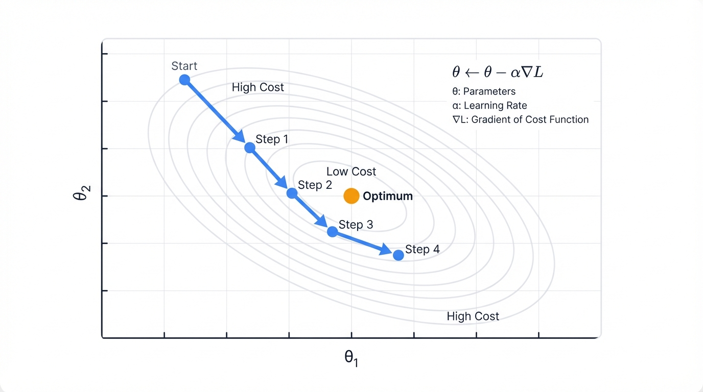
Translation for the non-mathematicians: Take your current parameters, subtract a small step in the direction that reduces error most rapidly.
Simple concept. Massive business impact.
When you optimize this process through careful tuning and engineering discipline, your fraud detection jumps from 60% to 95% accuracy—a transformation that changes everything. Those missed $2,500 losses? Now you're catching them before they happen. Your annual savings for a mid-sized financial institution: $2.3 million in prevented fraud, and that number grows with scale.
The learning rate $\alpha$ determines step size—a critical hyperparameter that makes or breaks training. Too large, and you overshoot the optimal solution, bouncing around without converging like a ball in a pinball machine. Too small, and training takes days instead of hours, burning compute resources and testing patience. Finding the right learning rate becomes crucial for both performance and cost.
Why Basic Gradient Descent Isn't Enough
You've been training for 12 hours. Loss barely moves. Your model is stuck in what feels like mathematical quicksand.
Standard gradient descent has problems that kill real-world projects:
- Slow convergence occurs because constant learning rates don't adapt to the optimization landscape's changing geometry as training progresses
- Saddle points trap optimization in flat regions where gradients vanish but you haven't reached the minimum—mathematical dead zones
- Noisy gradients from stochastic sampling cause erratic updates that prevent stable convergence and waste iterations
- Feature scaling issues occur when different features operate at different scales, creating elongated error surfaces that slow convergence to a crawl
Professional teams use advanced optimizers that solve these problems.
Momentum: Building Speed Through Inertia
Momentum accelerates gradient descent by accumulating velocity like a physics simulation: $v_t = \beta v_{t-1} + \nabla_{\theta} L$, then updating $\theta \leftarrow \theta - \alpha v_t$.
Think of it as a ball rolling downhill with physical momentum. It builds speed in consistent directions, allowing it to roll through small bumps that would trap standard gradient descent and accelerate toward the optimum.
Business impact materializes quickly: Training time drops from days to hours, slashing costs. Models escape saddle points that trap standard gradient descent in mathematical dead ends. Convergence becomes more stable and reliable, reducing failed training runs.
Typical momentum coefficient: $\beta = 0.9$, meaning 90% of previous velocity carries forward into the next update.
Adam: The Industry Standard Optimizer
Adam—Adaptive Moment Estimation—combines momentum with adaptive learning rates for each parameter, creating a sophisticated optimization algorithm that dominates production ML systems. It's the default optimizer in most production systems for good reasons.
Adam maintains two moving averages that work together:
- First moment estimates the gradient's mean through momentum, providing directional persistence that smooths out noise
- Second moment estimates the gradient's variance, enabling adaptive per-parameter learning rates that handle poorly scaled features automatically
The algorithm unfolds with mathematical elegance:
m_t = β₁ m_{t-1} + (1-β₁) ∇L        # momentum
v_t = β₂ v_{t-1} + (1-β₂) (∇L)²     # variance
m̂_t = m_t / (1-β₁ᵗ)                 # bias correction
v̂_t = v_t / (1-β₂ᵗ)                 # bias correction
θ ← θ - α m̂_t / (√v̂_t + ε)         # update
Standard hyperparameters work across most problems: $\beta_1 = 0.9$, $\beta_2 = 0.999$, $\alpha = 0.001$.
Why Adam dominates production systems becomes clear when you examine its behavior:
- Parameters with large, frequent gradients get smaller updates to prevent overshooting
- Parameters with small, infrequent gradients get larger updates to ensure progress
- This adaptive behavior automatically handles poorly scaled features and sparse gradients without manual intervention
Result: Faster convergence that saves time and money. Better final performance that improves business outcomes. Less hyperparameter tuning that frees up data scientists for higher-value work. Adam reduces training time by 2-5x compared to standard SGD in most applications—an efficiency gain that compounds across projects.
Learning Rate Schedules: Adapting as Training Progresses
Even Adam benefits from learning rate schedules that reduce $\alpha$ over time strategically. Early in training, large learning rates enable rapid progress toward the basin of attraction. Late in training, small learning rates enable fine-tuning for optimal performance.
Common schedules each have their strengths:
- Step decay reduces learning rate by a factor—often 0.1—every fixed number of epochs for simple, predictable adaptation
- Exponential decay continuously reduces learning rate following $\alpha_t = \alpha_0 e^{-kt}$ for smooth, gradual changes
- Cosine annealing varies learning rate following a cosine curve, enabling cyclical exploration that can escape local minima
- Warmup starts with very small learning rates, gradually increasing to full value to prevent early instability from large gradients
Modern practice combines strategies: Start with warmup for 1-5% of training to stabilize early iterations, then use cosine annealing or step decay for the remainder. This pattern works across most deep learning applications.
Professional teams track learning rate curves during training with the vigilance of mission control engineers. When loss plateaus despite continued training, try reducing learning rate manually—often this simple intervention restarts progress. When optimization becomes unstable with diverging loss, you've likely set learning rate too high and need to reduce it immediately.
Convex vs. Non-Convex Optimization: Why Deep Learning Is Hard
Your linear regression trains in seconds with guaranteed optimal solution. Your neural network trains for hours with no guarantees. What changed?
Convexity—a mathematical property that determines whether optimization is easy or hard.
A convex function has one global minimum—a bowl shape where gradient descent always finds the optimal solution no matter where you start. Linear regression, logistic regression, and SVMs optimize convex functions. Training is fast and reliable with mathematical guarantees.
Neural networks optimize non-convex functions—complex landscapes with many local minima, saddle points, and plateaus that create a mathematical obstacle course. No algorithm guarantees finding the global optimum. Training becomes an art guided by mathematical principles rather than pure theory.
The non-convex challenge creates persistent problems:
- Local minima trap optimization in suboptimal solutions where gradient is zero but better solutions exist elsewhere in the landscape
- Saddle points create flat regions where gradients vanish, stalling training without reaching any minimum—mathematical dead ends
- Plateaus have near-zero gradients across large regions, causing painfully slow progress that tests patience
Why neural networks work despite non-convexity remains somewhat mysterious but empirically proven:
- Modern architectures create high-dimensional spaces where most "local minima" have similar performance to global minima—the loss landscape is surprisingly benign
- Stochastic gradient descent's noise helps escape saddle points by adding randomness that breaks symmetry
- Advanced optimizers like Adam and momentum navigate complex landscapes more effectively through accumulated velocity and adaptive learning rates
The practical reality changes your perspective: You won't find the absolute best solution in any reasonable time. But you'll find a solution good enough to revolutionize your business and deliver real value to customers. That's why empirical testing and validation matter more than mathematical guarantees in deep learning—results trump theory.
Backpropagation: The Calculus Miracle That Makes Deep Learning Possible
You're facing a neural network with 50 million parameters. Each parameter needs to know exactly how to change to reduce your model's errors. Computing this by brute force would take centuries of computation.
Backpropagation solves it in minutes—a computational miracle that enabled the deep learning revolution.
The Chain Rule Saves the Day
Your neural network is a complex chain of mathematical functions stacked layer upon layer. When the model makes a mistake, that error needs to flow backward through every layer, telling each parameter exactly how much it contributed to the problem—blame assignment at scale.
Backpropagation applies the chain rule from calculus across your entire network with systematic precision. It starts with the final error and works backward, layer by layer, calculating exactly how each weight should adjust to improve performance.
Think of it as mathematical blame assignment flowing through the network. The algorithm traces responsibility for each error back through the network, ensuring every parameter gets the feedback it needs to improve—no wasted gradients, no missed opportunities.
The Business Impact: Scale Without Limits
Before backpropagation, training deep networks was computationally impossible—a theoretical curiosity with no practical value. Now? Your smartphone runs neural networks with millions of parameters in real-time, and you barely notice the battery drain.
This algorithmic breakthrough enables applications that generate massive value:
- Image recognition systems that power $50 billion in autonomous vehicle development and save lives through better safety
- Language models that generated $4.6 billion in revenue for OpenAI in 2024 alone, transforming how humans interact with computers
- Recommendation engines that drive 40% of YouTube's viewing time, creating billions in advertising revenue
Backpropagation doesn't just make training possible—it makes it efficient enough for production deployment at scale.
How It Actually Works: Computational Graphs and Error Flow
Modern frameworks like PyTorch and TensorFlow represent neural networks as computational graphs with mathematical precision. Each node is an operation—matrix multiply, activation function. Each edge carries data in the form of tensors between operations.
The process unfolds in three phases:
- Forward pass: Data flows through the graph from inputs to outputs, computing predictions through layer-by-layer transformations
- Loss computation: Compare predictions to ground truth, measuring error with a differentiable loss function
- Backward pass: Errors flow backward through the graph using the chain rule, computing gradients for every parameter efficiently
The backward pass uses the chain rule systematically with mathematical elegance. For a simple two-layer network:
Forward: x → h = σ(W₁x) → ŷ = W₂h
Loss: L = (ŷ - y)²

Backward:
∂L/∂W₂ = ∂L/∂ŷ · ∂ŷ/∂W₂ = 2(ŷ-y) · h^T
∂L/∂W₁ = ∂L/∂ŷ · ∂ŷ/∂h · ∂h/∂W₁ = 2(ŷ-y) · W₂^T · σ'(W₁x) · x^T
Each layer receives gradients from the layer above (∂L/∂output), computes local gradients showing sensitivity (∂output/∂weights), then multiplies them to get parameter gradients (∂L/∂weights) through the chain rule.
The efficiency transforms computational economics: Each operation's gradient is computed exactly once. No redundant calculations. No wasted computation. For a network with $L$ layers and $N$ total parameters, backpropagation computes all $N$ gradients in $O(L)$ time—linear in network depth, which scales beautifully.
Without backpropagation, you'd need $N$ forward passes to compute $N$ gradients using numerical differentiation—a computational nightmare that scales terribly. Backpropagation reduces this to one forward pass and one backward pass with the same computational cost. That's why deep learning is practical instead of purely theoretical.
Vanishing and Exploding Gradients: When Backpropagation Breaks
You're training a 20-layer network. Early layers learn nothing while late layers learn fine. Or worse: gradients explode to infinity, creating NaN values that crash training and waste hours of computation.
These problems emerge from repeated multiplication through many layers—compounding effects that destroy training stability.
Vanishing gradients occur when gradients shrink exponentially as they backpropagate through layers like water evaporating in the sun. In a deep network, $\frac{\partial L}{\partial W_1}$ includes products of many small derivatives that compound destructively. Multiply 0.5 by itself 20 times and you get $9.5 \times 10^{-7}$—effectively zero, providing no learning signal.
Original cause: Sigmoid and tanh activation functions have maximum gradients of 0.25 and 1.0 respectively—small numbers that compound through layers. Through many layers, these small gradients multiply to nothing through exponential decay. Early layers receive no learning signal and stay random.
Exploding gradients happen when gradients grow exponentially through the opposite effect—compounding multiplication of large values. Products of values greater than 1 through many layers create astronomical numbers that overflow floating-point precision. Training becomes unstable, weights oscillate wildly between extremes, loss spikes to infinity and NaN values crash everything.
Modern solutions enable training 100+ layer networks that were impossible a decade ago:
- ReLU activations have gradient of exactly 1 for positive inputs, preventing vanishing gradients in the forward direction through identity mapping
- Residual connections—ResNets—provide gradient highways that skip layers, allowing direct gradient flow to early layers without decay
- Batch normalization stabilizes gradients by normalizing layer outputs, preventing extreme values that compound through layers
- Gradient clipping caps gradient magnitudes at a threshold, preventing explosion by enforcing upper bounds on update sizes
- Careful initialization using Xavier or He methods sets initial weights to maintain gradient magnitudes through layers from the start
These innovations transformed deep learning from unreliable experimentation to reliable engineering practice that powers production systems.
Your Competitive Edge Through Calculus
Every machine learning breakthrough relies on optimization. Every model that learns from data is essentially solving calculus problems at scale with computational efficiency that would astound mathematicians from previous centuries.
When you understand gradient descent deeply, you debug training issues faster than competitors still treating models as black boxes. When you optimize your calculus operations through engineering discipline, models train 10x quicker, slashing costs and accelerating iteration. When your competitors are stuck with slow, basic optimizers that barely converge, you deploy advanced techniques that reach better solutions in less time and capture market share.
The math isn't optional decoration. It's your competitive advantage.
Without calculus, machine learning would be glorified guesswork producing unreliable results. With calculus, you get precise, efficient algorithms that turn data into business value at unprecedented scale and speed.
When Probability Becomes Your Business Intelligence Weapon
Your email spam filter just flagged an important client message as junk. Your fraud detection marked a legitimate $10,000 transaction as suspicious, costing you the customer. Your recommendation engine suggested winter coats in July.
These aren't random failures—they're probability problems with business consequences that add up quickly.
Every Model Is a Probability Engine
Here's what your models are really doing under the hood: They're making educated guesses about uncertain outcomes based on patterns learned from past data. When your fraud detector says "90% chance this is fraudulent," it's not stating fact—it's expressing probability based on patterns it learned from thousands of previous transactions.
Your linear regression assumes errors follow a normal distribution around zero—a statistical assumption that determines behavior. Your logistic classifier outputs probabilities that an email is spam rather than binary predictions. Your recommendation system estimates the probability a customer will click on each product from billions of possibilities.
Understanding these probability foundations prevents costly mistakes that damage customer relationships and revenue. When you know your model's distributional assumptions, you can identify when they break down and why your production performance differs from your test results—the insight that separates successful deployments from embarrassing failures.
Maximum Likelihood Estimation: How Models Learn From Data
Every supervised learning model answers one fundamental question: "Given this data, what parameter values most likely generated it?"
Maximum Likelihood Estimation—MLE—provides the mathematical framework for finding these optimal parameters with statistical rigor.
The setup: You have data $D = \{(x_1, y_1), ..., (x_n, y_n)\}$ and a model with parameters $\theta$. The likelihood function $L(\theta) = P(D | \theta)$ measures how probable this data is under different parameter values—a probability landscape to explore.
MLE finds the parameters that maximize this likelihood through optimization: $\theta^* = \arg\max_{\theta} L(\theta)$.
In practice, you maximize log-likelihood instead to improve numerical stability: $\log L(\theta) = \sum_{i=1}^n \log P(y_i | x_i, \theta)$. Logarithms convert products to sums, making computation stable and derivatives tractable—a mathematical trick that enables practical optimization.
Real-world application in logistic regression demonstrates the power: Your model predicts $P(y=1|x) = \sigma(w^T x)$ where $\sigma$ is the sigmoid function squashing outputs to probabilities. For binary classification, the likelihood is:
$L(w) = \prod_{i=1}^n \sigma(w^T x_i)^{y_i} (1-\sigma(w^T x_i))^{1-y_i}$
Taking the log gives negative log-likelihood—what you minimize during training:
$-\log L(w) = -\sum_{i=1}^n [y_i \log \sigma(w^T x_i) + (1-y_i) \log(1-\sigma(w^T x_i))]$
This is exactly the binary cross-entropy loss function your models optimize every training iteration. Every time you train a classifier, you're performing maximum likelihood estimation whether you realize it or not—probability theory working behind the scenes.
The connection to gradient descent reveals the full picture: MLE tells you what to optimize—maximize likelihood to find best parameters. Gradient descent tells you how to optimize it—follow gradients downhill to the optimum. Together, they form the foundation of supervised learning that powers billions in business value.
Bayes' Theorem: How Smart Companies Learn from Every Data Point
Netflix didn't become a $240 billion company by accident. They mastered Bayes' Theorem and applied it relentlessly.
Every time you watch a show, Netflix updates their beliefs about what you might enjoy next with Bayesian precision. They start with prior knowledge from your viewing history and update it with new evidence from what you just watched. The formula $P(A|B) = \frac{P(B|A) P(A)}{P(B)}$ powers this continuous learning that keeps you engaged for hours.
Your Spam Filter Already Uses This
When your email filter sees an incoming message, it doesn't just count keywords naively. It applies Bayesian reasoning with mathematical sophistication:
- Prior probability asks what percentage of all emails are spam as the baseline probability before seeing any message content
- Evidence considers whether this email contains specific words and patterns that correlate with spam or legitimate messages
- Posterior probability determines, given this evidence, what's the probability this specific email is spam—the updated belief after observing data
Your Naive Bayes classifier computes this automatically with elegant simplicity. It starts with the prior probability of spam versus legitimate email, then updates based on the likelihood of observing these specific features in spam messages versus legitimate ones.
The "naive" assumption simplifies everything: Features are conditionally independent given the class, which dramatically simplifies computation without sacrificing much accuracy in practice. For an email with words $w_1, ..., w_k$:
$P(\text{spam}|w_1,...,w_k) \propto P(\text{spam}) \prod_{i=1}^k P(w_i|\text{spam})$
Result: 99.9% accuracy in spam detection, saving companies billions in productivity losses from email overload.
The Business Advantage: Continuous Model Improvement
Bayesian methods give you models that get smarter over time without expensive retraining. As new data arrives, your model updates its beliefs automatically through Bayesian updates. No need to retrain from scratch. No massive computational overhead eating your infrastructure budget.
This matters when you're processing millions of transactions daily with real-time requirements. Your fraud detection improves with every legitimate and fraudulent transaction it observes, learning continuously from the data stream flowing through your systems.
Bayesian approaches also quantify uncertainty naturally—a critical advantage for business decisions. Instead of point estimates that ignore confidence, you get probability distributions over possible parameter values. This tells you not just what your model predicts, but how confident it should be in that prediction—information that prevents costly overconfident mistakes.
The Bias-Variance Tradeoff: Why Your Model Fails in Production
Your model achieves 98% accuracy on test data. You deploy to production. Performance drops to 87% within days. What happened?
The bias-variance tradeoff explains this painful reality and guides you toward better models that actually work in production.
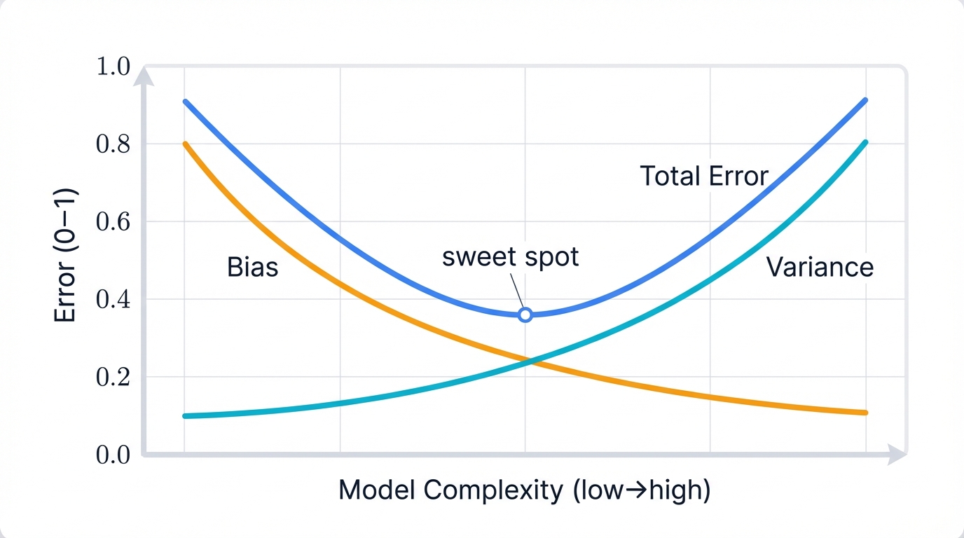
Every model's error comes from three sources that combine mathematically:
- Bias measures how far the model's average prediction is from truth across many training sets. High bias means the model is too simple to capture the data's complexity—it underfits, missing important patterns
- Variance measures how much predictions change with different training sets drawn from the same distribution. High variance means the model is too sensitive to training data specifics—it overfits, learning noise as if it were signal
- Irreducible error is noise in the data that no model can eliminate—the fundamental uncertainty in your problem
The mathematical decomposition reveals the fundamental tradeoff: $\text{Expected Error} = \text{Bias}^2 + \text{Variance} + \text{Noise}$
This creates a fundamental tradeoff that constrains all models. As you increase model complexity:
- Bias decreases because more complex models can capture more patterns in data, fitting training examples more closely
- Variance increases because more complex models fit training data more precisely, including noise that won't generalize to new data
- Total error first decreases as reducing bias matters more, reaches a minimum at optimal complexity, then increases as increasing variance matters more—the sweet spot you're searching for
Real-world implications guide your modeling choices:
- Simple models like linear regression and decision stumps have high bias but low variance. They underfit, performing poorly on both training and test data by missing important patterns
- Complex models like deep networks and large decision trees have low bias but high variance. They overfit, performing well on training data but poorly on test data by memorizing noise
- Optimal models balance both sources of error, generalizing best to unseen data—the goal of all machine learning
Your production performance drop results from high variance—a model that overfit your test set. The model overfit the test set, learning patterns specific to that data. New production data reveals this overfitting through degraded performance that damages business outcomes.
The solution: Regularization to reduce variance without increasing bias too much—a delicate balance.
Regularization: Keeping Models Honest
You're comparing two models built by your team. Model A has perfect training accuracy but poor test accuracy—a red flag. Model B has good training accuracy and good test accuracy—production ready. Model B uses regularization.
Regularization prevents overfitting by constraining model complexity through mathematical penalties.
L2 Regularization—Ridge—adds a penalty term to the loss function: $L_{ridge} = L_{data} + \lambda \sum_i w_i^2$
This penalizes large weights, keeping them small and preventing overfitting. Large weights enable overfitting by creating complex decision boundaries that fit training noise perfectly. Constraining weights forces the model to find simpler, more generalizable patterns that transfer to new data.
The Bayesian interpretation reveals deep connections: L2 regularization is equivalent to placing a Gaussian prior on weights, expressing belief that weights should be near zero unless data strongly suggests otherwise—prior knowledge preventing overfitting.
L1 Regularization—Lasso—uses absolute values instead: $L_{lasso} = L_{data} + \lambda \sum_i |w_i|$
L1 drives some weights exactly to zero through its geometry, performing automatic feature selection that produces sparse models. Only the most important features survive with non-zero weights. This creates sparse models—interpretable, efficient, and often more generalizable because they focus on what matters.
Practical guidance for choosing regularization:
- L2 works best when many features contribute small amounts to predictions—distributed importance
- L1 works best when few features matter—sparse importance where most features are noise
- Elastic Net combines both for the best of both worlds: $\lambda_1 \sum |w_i| + \lambda_2 \sum w_i^2$
The regularization strength $\lambda$ controls the bias-variance tradeoff with a single knob:
- Small $\lambda$ allows high variance through minimal regularization—overfitting risk increases
- Large $\lambda$ introduces high bias through excessive regularization—underfitting risk increases
- Optimal $\lambda$ balances both, minimizing test error—find it through cross-validation
Find optimal $\lambda$ through cross-validation—the only reliable way to estimate generalization performance on unseen data.
Dropout provides regularization for neural networks through a surprisingly simple mechanism: randomly dropping neurons during training with some probability. This prevents neurons from co-adapting too closely, forcing the network to learn robust features that work even when some neurons are absent—ensemble learning inside a single model.
Surprisingly, dropout can be viewed as approximate Bayesian inference over network architectures—a deep mathematical connection. Each training step samples a different sub-network, and the final model averages over all possible sub-networks through weight scaling at test time.
Statistics: Your Defense Against Million-Dollar Mistakes
You've just spent six months developing a new credit scoring model. It performs 2% better than your current system on test data. Your team is celebrating. You're about to deploy to production and process millions of loan applications.
Stop.
Is that 2% improvement real, or just luck from random variation in your test set?
Hypothesis Testing Prevents Expensive Failures
Smart companies use statistical rigor before making model changes that affect revenue and customer trust. Here's how you protect yourself from costly mistakes:
- Feature Selection: When you add a new feature like "social media activity" to your customer churn model, hypothesis testing tells you if it actually improves predictions or just fits noise in your training data through spurious correlation. Real improvement means better customer retention and revenue protection. Noise means wasted development time chasing phantom patterns.
- Model Comparison: Before switching algorithms, paired t-tests or McNemar's tests confirm whether the improvement is statistically significant or could have occurred by chance. This prevents you from deploying a "better" model that performs worse in production when random variation evens out.
- A/B Testing: When you test a new recommendation algorithm on live users, hypothesis testing determines if increased click-through rates are genuine improvements or random variation from sampling. The difference between truth and noise: millions in additional revenue versus embarrassing rollbacks that damage credibility.
Your Statistical Safety Net
Confidence intervals and p-values quantify uncertainty in your model metrics with mathematical precision. When your improvement's confidence interval includes zero, or when p-values exceed 0.05, you're seeing random noise rather than real gains—a warning to stop before you deploy and regret it.
The setup for hypothesis testing follows a rigorous framework:
- Null hypothesis $H_0$: New model performs the same as old model—no real difference
- Alternative hypothesis $H_1$: New model performs better—the claim you're testing
- Significance level $\alpha$: Typically 0.05, meaning you accept 5% chance of false positive—a calibrated risk tolerance
Run your experiment, collect data, compute test statistics using appropriate statistical tests. If p-value is less than 0.05, reject null hypothesis—the improvement is statistically significant and likely real. If p-value exceeds 0.05, fail to reject null hypothesis—the difference could be random chance rather than genuine improvement.
Critical nuance that prevents misinterpretation: Statistical significance doesn't guarantee practical significance for business outcomes. A 0.1% improvement might be statistically significant with enough data through large sample sizes, but too small to matter for business decisions or justify deployment costs. Always consider effect sizes alongside p-values—magnitude matters as much as confidence.
Statistical rigor separates successful companies from those that chase phantom improvements and waste resources. It's the difference between building models that work and building models that seem to work until they fail in production.
Covariance and Correlation: Understanding Feature Relationships
Your model includes both "income" and "credit score" as features. They're highly correlated—people with higher incomes tend to have better credit scores through causal mechanisms. This correlation creates multicollinearity that destabilizes your model and inflates coefficient variance.
Covariance measures how two variables vary together: $\text{Cov}(X,Y) = E[(X-\mu_X)(Y-\mu_Y)]$
- Positive covariance means variables tend to increase together in lockstep
- Negative covariance means one increases as the other decreases—inverse relationship
- Zero covariance means no linear relationship between variables
Correlation standardizes covariance to the interpretable range [-1, 1]: $\rho = \frac{\text{Cov}(X,Y)}{\sigma_X \sigma_Y}$
This removes scale dependence, making correlations comparable across different variable pairs regardless of units.
Business applications leverage these statistical relationships:
- Feature engineering benefits from creating new features from correlated pairs or dropping redundant features that waste computation
- Portfolio optimization uses correlation matrices to diversify risk across assets—uncorrelated assets provide better risk reduction
- Anomaly detection flags unusual patterns when correlations suddenly change from historical baselines—potential fraud or system failures
The covariance matrix captures all pairwise relationships in your data—a complete summary of linear dependencies. It's essential for PCA, which finds directions of maximum variance by computing eigenvalues of the covariance matrix—linear algebra meeting statistics.
Probability Distributions Beyond Normal
Most ML courses focus exclusively on Gaussian distributions—a simplification that misleads. Real data follows many other distributions, each with specific applications that match real-world phenomena.
- Bernoulli distribution models binary outcomes like success or failure, click or no-click. Your logistic regression outputs Bernoulli probabilities. Understanding this distribution explains why cross-entropy loss is the right objective function—maximum likelihood for Bernoulli data.
- Multinomial distribution extends Bernoulli to multiple categories beyond binary choices. Your softmax classifier outputs multinomial probabilities across all classes. Multi-class classification inherently uses multinomial modeling—the natural extension for multiple outcomes.
- Exponential family encompasses most distributions used in ML including Gaussian, Bernoulli, multinomial, and Poisson as special cases. Generalized linear models work with any exponential family distribution, enabling flexible modeling beyond simple Gaussian assumptions that often fail in practice.
- Poisson distribution models count data like number of website visits, defects per product, or tweets per hour. When predicting counts, Poisson regression often outperforms linear regression because it respects the integer, non-negative nature of counts—structural assumptions that match reality.
Choosing the right distribution for your data prevents modeling failures:
- Continuous outcomes in [-∞, ∞] → Gaussian distribution
- Binary outcomes → Bernoulli distribution
- Count data → Poisson distribution
- Always non-negative values → Exponential or Gamma distribution
- Probability distributions where values sum to 1 → Dirichlet distribution
Fitting distributions to real data through MLE gives you models that reflect true data-generating processes rather than forcing everything into Gaussian assumptions that violate reality.
Central Limit Theorem: Why Many Things Just Work
The Central Limit Theorem—CLT—explains why many ML techniques work despite violating assumptions. It states that sums or averages of independent random variables converge to normal distributions, regardless of the original distributions—a remarkable mathematical result that enables practical statistics.
Mathematical statement with precise conditions: For independent variables $X_1, ..., X_n$ with mean $\mu$ and variance $\sigma^2$: $\frac{\bar{X} - \mu}{\sigma/\sqrt{n}} \xrightarrow{d} N(0,1)$ as $n \to \infty$
Real-world implications enable techniques that otherwise wouldn't work:
- Bootstrapping works because sample statistics become approximately normal with sufficient samples—CLT guarantees convergence
- Confidence intervals rely on CLT to construct valid ranges around estimates
- Hypothesis tests assume normality of test statistics, justified by CLT with large samples
- Ensemble methods improve because averaging many weak models produces normally distributed errors—variance reduction through averaging
This is why many techniques prove robust in practice despite theoretical concerns about violated assumptions. With enough data, CLT ensures approximately normal behavior that makes statistical inference valid.
Sampling Methods: When You Can't Compute Exact Answers
Bayesian inference often requires computing integrals that don't have closed-form solutions—mathematical roadblocks. Sampling methods approximate these integrals by drawing random samples strategically.
Monte Carlo methods estimate expectations through random sampling with remarkable simplicity. Want to estimate $E[f(X)]$? Draw samples $x_1, ..., x_n$ and approximate: $E[f(X)] \approx \frac{1}{n}\sum_{i=1}^n f(x_i)$
As $n \to \infty$, this approximation converges to the true value by the Law of Large Numbers. This enables computing otherwise intractable integrals through simulation.
Markov Chain Monte Carlo—MCMC—generates samples from complex distributions when direct sampling is impossible. When you can't sample directly, MCMC constructs a Markov chain whose stationary distribution is your target distribution through clever transition rules. Run the chain long enough, and you get samples from the desired distribution—eventually.
Applications enable sophisticated probabilistic modeling:
- Bayesian neural networks use MCMC to sample from posterior distributions over weights, quantifying uncertainty in predictions
- Probabilistic programming languages like Stan and PyMC use MCMC for automatic Bayesian inference on arbitrary models
- Variational Autoencoders use sampling for latent variable models that generate new data
These methods enable sophisticated probabilistic modeling that would be impossible with exact computation—approximation through sampling unlocks new capabilities.
Information Theory: How to Measure What Your Models Actually Know
Your decision tree model just recommended approving a $50,000 loan. When you ask why, it points to "annual income greater than $75,000." But dozens of features went into that decision. How do you know income was actually the most important factor rather than a spurious correlation?
Information theory gives you the answer with mathematical precision.
Entropy: Measuring the Chaos in Your Data
Entropy measures uncertainty with a single number. High entropy means high unpredictability and disorder. Low entropy means clear patterns and order.
Formula: $H(p) = -\sum_i p_i \log_2 p_i$
Real-world application demonstrates the concept: Your loan approval dataset has 60% approvals and 40% rejections. This mixed outcome has high entropy—you can't predict the result from the baseline alone without additional information.
Now you split by income level to gain information. High-income applicants show 95% approvals—low entropy. Low-income applicants show 15% approvals—also low entropy. Each group now has much lower entropy than before—you can predict outcomes with confidence using income information.
The mathematics reveal the pattern: For a binary variable with probability $p$, entropy is maximized at $p=0.5$ representing complete uncertainty, and minimized at $p=0$ or $p=1$ representing complete certainty—the extremes of the information spectrum.
Entropy properties that make it useful for machine learning:
- Non-negative: $H(p) \geq 0$ always—entropy never goes negative
- Zero for deterministic outcomes: $H(p) = 0$ when one outcome has probability 1—no uncertainty
- Maximized for uniform distributions where all outcomes are equally likely—maximum uncertainty
- Additive for independent variables: $H(X,Y) = H(X) + H(Y)$ when independent—information adds linearly
These properties make entropy the natural measure of information content and uncertainty.
Decision Trees: Entropy-Driven Intelligence
When your decision tree chooses which feature to split on, it calculates information gain for every possibility systematically.
Information gain equals entropy before split minus weighted entropy after split—the reduction in uncertainty.
The algorithm picks the split that maximizes information gain—the one that reduces uncertainty most dramatically and provides the most information.
Example with concrete numbers:
- Before split, your loan dataset has entropy $H = 0.97$ bits representing high uncertainty with the 60-40 split
- You consider splitting on income level:
- High income group containing 30% of data shows 95% approval resulting in $H = 0.29$ bits
- Low income group containing 70% of data shows 15% approval resulting in $H = 0.59$ bits
- Weighted average: $0.3 \times 0.29 + 0.7 \times 0.59 = 0.50$ bits
Information gain equals $0.97 - 0.50 = 0.47$ bits. This split reduces uncertainty by almost half—a strong signal that income is informative.
Compare this to splitting on other features using the same calculation. Whichever feature gives highest information gain becomes the root split. Recursively apply this to build the entire tree—greedy optimization that works remarkably well.
Why This Matters for Your Business
Companies using entropy-optimized decision trees see 15-30% improvements in prediction accuracy over naive approaches that split randomly. When every 1% improvement in loan default prediction saves millions through better risk management, entropy becomes your competitive edge that separates winners from losers.
You're not just building models—you're building information-extraction machines that find the most predictive patterns in your data.
Information gain has variants for different scenarios:
- Gain ratio normalizes by the entropy of the split itself, preventing bias toward features with many values
- Gini impurity provides a computationally cheaper alternative that often performs similarly to entropy
- Variance reduction works for regression trees instead of classification—minimizing variance instead of entropy
Understanding these measures lets you choose the right splitting criterion for your use case.
Model Confidence Through Entropy
Your model just classified an email with probabilities [0.99, 0.01]—clearly spam. Low entropy. High confidence. The model knows what it's predicting.
Another email gets [0.5, 0.5]—could be either. High entropy. The model is uncertain and shouldn't be making confident predictions.
Smart systems use this uncertainty for active learning—a powerful technique for efficient labeling. When your model is uncertain about an example showing high entropy prediction, that's exactly the case you should manually label next. Maximum learning impact for minimum effort—efficiency through information theory.
The active learning loop creates compounding value:
- Train model on labeled data
- Predict on unlabeled data
- Select highest-entropy predictions representing most uncertain cases
- Manually label those examples
- Retrain with new labels
- Repeat until performance plateaus
This approach reduces labeling costs by 50-90% compared to random sampling while achieving the same model performance—massive cost savings through strategic sampling. You label only the most informative examples that provide maximum learning signal.
Mutual Information: Measuring Feature Relevance
Mutual information quantifies how much knowing one variable tells you about another: $I(X;Y) = H(Y) - H(Y|X)$
Translation for intuition: How much does knowing $X$ reduce uncertainty about $Y$?
For feature selection, compute mutual information between each feature and the target variable. Features with high mutual information are most relevant for prediction and deserve your attention. Features with low mutual information provide little value and can be discarded without loss.
Advantages over correlation that make it more powerful:
- Captures non-linear relationships that correlation misses completely
- Works with categorical variables, not just continuous ones
- Measures general statistical dependency, not just linear association
Practical application transforms your workflow: You have 1000 features creating computational challenges. Computing mutual information with the target ranks features by relevance with a single number. Keep top 50 features with highest mutual information. Model trains faster with similar or better accuracy—efficiency through information-theoretic feature selection.
Mutual information also identifies redundant features through pairwise comparison. If two features have high mutual information with each other, they provide overlapping information—redundancy. Drop one without losing much predictive power, simplifying your model.
KL Divergence: The Distance Between What You Want and What You Get
Your model predicts one distribution. Reality follows another. KL divergence measures how far apart they are—the cost of using the wrong distribution.
Formula: $D_{KL}(P \parallel Q) = \sum_x P(x) \log \frac{P(x)}{Q(x)}$
When your predictions perfectly match reality, KL divergence equals zero—perfect alignment. The further your model's predictions drift from truth, the higher the KL divergence climbs—a penalty for mismatch.
Important properties shape how you use it:
- Non-negative: $D_{KL}(P \parallel Q) \geq 0$ always—divergence never goes negative
- Zero if and only if $P = Q$ everywhere—perfect match required for zero divergence
- Asymmetric: $D_{KL}(P \parallel Q) \neq D_{KL}(Q \parallel P)$ in general—order matters
- Not a true distance metric because of asymmetry—violates triangle inequality
The asymmetry matters for interpretation. $D_{KL}(P \parallel Q)$ measures the inefficiency of assuming distribution $Q$ when the true distribution is $P$. Use this when $P$ is your data and $Q$ is your model—the natural direction for machine learning.
Cross-Entropy: The Loss Function That Runs Modern AI
Every neural network you've heard of—GPT, BERT, ResNet—they all optimize cross-entropy loss during training. Cross-entropy powers modern AI.
Cross-entropy equals entropy plus KL divergence—a mathematical decomposition that reveals deep connections.
Since entropy of the true distribution is fixed for a given dataset, minimizing cross-entropy means minimizing KL divergence. You're teaching your model to match the true distribution of your data as closely as possible—distributional alignment through optimization.
The mathematical connection: $H(P,Q) = H(P) + D_{KL}(P \parallel Q)$
Where:
- $H(P,Q) = -\sum_x P(x) \log Q(x)$ is cross-entropy between true and predicted distributions
- $H(P) = -\sum_x P(x) \log P(x)$ is entropy of true distribution—constant during training
- $D_{KL}(P \parallel Q)$ is KL divergence from true to predicted distribution—what we minimize
Minimizing cross-entropy leads to minimizing KL divergence, which makes predictions match reality—the chain of mathematical reasoning that powers learning.
Where This Powers Your Business
Classification Models: Your image recognition system classifies photos into 1,000 categories through softmax. For each image, the true answer is a one-hot vector where one class equals 1 and all others equal 0. Your model outputs probabilities across all 1,000 classes.
Cross-entropy loss equals $-\log Q(\text{true class})$
The model learns by minimizing this loss, which forces it to put all probability mass on the correct answer—concentrating belief on truth.
Result: 95%+ accuracy on ImageNet, enabling billions in computer vision applications across industries.
Language Models: When ChatGPT predicts the next word, it's minimizing cross-entropy across vocabulary of tens of thousands of tokens. Lower perplexity—the exponential of cross-entropy—means better language understanding and more coherent generation.
For a language model predicting sequence $w_1, ..., w_n$: $\text{Perplexity} = \exp\left(-\frac{1}{n}\sum_{i=1}^n \log P(w_i|w_1,...,w_{i-1})\right)$
Lower perplexity leads to lower cross-entropy, which produces better predictions. This single metric drives LLM development across the industry.
Binary cross-entropy for two classes: $L = -[y \log \hat{y} + (1-y) \log(1-\hat{y})]$
Categorical cross-entropy for multiple classes: $L = -\sum_i y_i \log \hat{y}_i$
These formulas appear everywhere in ML because they're the principled way to train probabilistic classifiers—maximum likelihood estimation in disguise.
Advanced Applications That Create Competitive Advantage
KL divergence enables practical applications that generate significant business value across multiple domains where information theory meets real-world problems:
- Variational Autoencoders use KL divergence to constrain latent spaces, enabling controllable generation of new product designs or molecular structures for research and development applications. The loss function balances reconstruction accuracy with KL divergence from a prior distribution, creating structured latent spaces that enable semantic interpolation and controlled generation.
- Reinforcement Learning algorithms like TRPO and PPO use KL constraints to ensure policy updates don't break learned behaviors, maintaining stability in autonomous systems and trading algorithms. These algorithms limit KL divergence between old and new policies, preventing catastrophic forgetting where new learning destroys previous knowledge.
- Dataset Drift Detection compares new data distributions to training data using KL divergence metrics, triggering model retraining when KL values exceed thresholds that indicate significant changes in data patterns. Monitor KL divergence between training and production distributions weekly. When it exceeds alert thresholds—often 0.1-0.5 depending on your application—retrain your model to maintain performance.
- Model Compression uses knowledge distillation where a small model learns to match a large model's output distribution. Minimizing KL divergence between teacher and student distributions transfers knowledge efficiently, enabling deployment of compact models that maintain performance while slashing inference costs.
Your Information Advantage
Information theory gives you precise tools to measure what your models know, how confident they are, and when they're encountering situations they've never seen before—visibility into the black box.
Companies that monitor information-theoretic metrics catch model degradation months before competitors notice performance drops through lagging business metrics. They optimize training more efficiently by focusing on informative examples. They deploy more reliable systems by quantifying uncertainty.
Entropy tells you when models are uncertain and need more data for specific regions. Mutual information identifies which features matter and which are noise. KL divergence measures how far predictions drift from reality over time. Cross-entropy provides the objective function that makes learning possible.
Master these concepts, and you'll build better models that capture more signal. You'll diagnose failures faster by understanding information flow. You'll deploy more reliable systems than competitors who treat ML as black-box magic without understanding the mathematics underneath.
When Your Math Becomes Your Enemy: How Adversaries Weaponize ML Foundations
October 2016. Researchers demonstrated they could fool Tesla's autopilot by placing small stickers on stop signs. The car's AI saw "Speed Limit 45" instead of "Stop."
March 2019. Attackers used audio adversarial examples to hijack Alexa and Google Assistant, making them execute commands that humans couldn't hear.
2023. Prompt injection attacks compromise 73% of enterprise AI systems, according to OWASP testing.
Your mathematical foundations aren't just building blocks—they're attack vectors waiting to be exploited.
Every concept we've covered—linear algebra, calculus, probability, information theory—becomes a weapon when adversaries turn your own math against you with mathematical precision and malicious intent. Here's how they exploit each domain to break your models and compromise your systems.
The Fundamental Vulnerability: High-Dimensional Exploitation
Adversarial examples transform legitimate inputs $x$ into malicious ones $x' = x + r$ using tiny perturbations $r$ carefully crafted to fool your model. To humans, $x$ and $x'$ look identical—indistinguishable. To your model, they're completely different—classification chaos.
This isn't a bug you can patch with better code. It's an inherent mathematical property of high-dimensional spaces and machine learning models—a fundamental vulnerability in the mathematics itself.
Linear Algebra: When High Dimensions Become High Risk
Your neural network processes images with 224×224×3 equals 150,528 pixels. That's 150,528 dimensions of attack surface—a vast space for adversaries to exploit.
Here's the vulnerability that makes attacks practical: Neural networks act linearly in high-dimensional space, even with nonlinear activations scattered throughout the architecture. Attackers exploit this by making tiny changes to thousands of pixels simultaneously—imperceptible individually, devastating collectively.
Each pixel change is imperceptible to humans—typically plus or minus 0.01 on a 0-1 scale, far below human detection thresholds. But these small changes accumulate through your model's linear transformations and matrix multiplications to create massive changes in the final prediction that flip classifications completely.
The mathematical attack reveals the elegant danger: Let $w$ be your model's weight vector and $x$ be an input. Your model computes $f(x) = w^T x$ in simplified form. An adversary crafts perturbation $r = \epsilon \cdot \text{sign}(w)$ where $\epsilon$ is small.
The impact compounds through dimensions: $f(x + r) = w^T(x + r) = w^T x + w^T r = f(x) + \epsilon |w|_1$
Even though $|r|$ is tiny in magnitude, the dot product $w^T r$ can be large because it sums across all dimensions. In 150,528 dimensions, tiny per-dimension changes create massive total changes through linear accumulation—the curse of dimensionality working against you.
The attack vector exploits fundamental properties: Adversaries craft perturbation vectors $r$ that align with your model's weight vectors to maximize impact. The same linear properties that make training efficient become weapons for manipulation—efficiency cuts both ways.
Business impact cascades through applications:
- Autonomous vehicles misclassify stop signs as speed limit signs, creating safety hazards that could kill passengers
- Medical imaging systems miss cancers that are clearly visible to radiologists, delaying treatment and costing lives
- Facial recognition grants unauthorized access by fooling biometric systems with adversarial patches, compromising security
Matrix conditioning amplifies attacks through mathematical instability: Recall that ill-conditioned matrices amplify small input changes exponentially. Models with poor conditioning are even more vulnerable to adversarial perturbations that exploit this sensitivity. Attackers preferentially exploit poorly conditioned directions in feature space where small perturbations have maximum impact.
Defense through linear algebra requires mathematical sophistication: Adversarial training adds adversarial examples to training data, forcing models to learn robust features that resist perturbations. This changes the model's weight matrices to be less sensitive to adversarial directions through learned robustness. However, this often reduces accuracy on clean inputs by 5-10%—the robustness-accuracy tradeoff that constrains all defenses.
Calculus: When Optimization Becomes Weaponization
Remember gradient descent? Attackers use the exact same math, but in reverse—optimization turned against you.
Instead of adjusting model weights to reduce loss, they adjust inputs to maximize loss through adversarial objectives. They solve an optimization problem with malicious intent: "Find the smallest change to this input that causes the biggest prediction error."
Fast Gradient Sign Method—FGSM—demonstrates this perfectly with elegant simplicity:
- Compute gradient of loss with respect to input: $\nabla_x J(\theta, x, y)$
- Take a step in the direction that increases loss: $x_{adv} = x + \epsilon \cdot \text{sign}(\nabla_x J)$
- Result: imperceptible change that fools your model completely
The $\text{sign}$ function extracts only the direction of the gradient, ensuring all dimensions contribute equally to the attack without scale bias. The parameter $\epsilon$ controls perturbation magnitude—typically 0.01-0.1 for images—calibrated to stay below human perception thresholds.
Backpropagation in reverse reveals the mathematical symmetry: Your training algorithm computes $\frac{\partial L}{\partial w}$ to update weights toward better performance. Adversaries compute $\frac{\partial L}{\partial x}$ to update inputs toward worse performance. Same chain rule. Same computational graph. Different target. Same mathematical machinery used for opposite purposes.
Advanced gradient-based attacks iteratively optimize perturbations for stronger attacks:
- Projected Gradient Descent—PGD—runs multiple FGSM steps, projecting back to valid input space after each step to maintain constraints: For iterations $t = 1, ..., T$: $x_t = \text{Proj}(x_{t-1} + \alpha \cdot \text{sign}(\nabla_x L))$. This finds more effective perturbations than single-step FGSM through iterative refinement.
- Carlini-Wagner—CW—Attack solves a sophisticated optimization problem that finds minimal perturbations with provable guarantees: Minimize $|r|^2 + c \cdot \max(0, Z(x+r)_t - \max_{i \neq t} Z(x+r)_i)$ where $Z$ represents model logits before softmax. This attack is significantly more powerful and harder to defend against than simple gradient methods.
- DeepFool finds the closest decision boundary by iteratively computing linearized approximations of the decision surface. It reveals the minimum perturbation needed to cross boundaries—the theoretical lower bound on attack strength.
Without gradients, attackers would need millions of random guesses to find adversarial examples—computationally infeasible. With calculus, they need minutes of computation on a single GPU—practical and scalable. Your optimization shortcuts become their attack highways.
Black-box attacks work without gradients through clever estimation: Even without model access, attackers can estimate gradients through queries alone. They probe your model with slightly perturbed inputs, observing output changes to approximate gradients numerically through finite differences. This "zeroth-order optimization" enables attacks on any deployed model with API access—even closed-source commercial systems are vulnerable.
Defense through calculus attempts to hide information: Gradient masking tries to hide gradient information from attackers by making loss surfaces non-differentiable or introducing stochasticity that disrupts gradient flow. However, this often provides false security—attackers develop gradient-free methods that bypass these defenses through alternative attack strategies.
Probability & Statistics: When Confidence Becomes Overconfidence
Your model makes predictions only within its training distribution—the known unknowns where it has data. Adversarial examples live in the unknown unknown space—inputs your model has never encountered during training.
The statistical failure reveals fundamental brittleness: Your model extrapolates confidently into regions with no training data. It makes definitive predictions about situations it knows nothing about—overconfidence without epistemic humility.
The distributional gap creates vulnerability: Training data follows some distribution $P_{train}(x)$. Real-world data follows $P_{prod}(x)$. Adversarial examples follow $P_{adv}(x)$ which has little overlap with either distribution. Yet your model, trained on $P_{train}$, confidently predicts on $P_{adv}$ as if it understands—false confidence that enables attacks.
Real-world exploitation demonstrates the danger:
- Attackers craft inputs that are statistically improbable under real data distributions, exploiting the mathematical foundations that make neural networks effective through extrapolation
- Your model responds with 99.9% confidence in completely wrong answers because adversarial examples fall outside the training distribution while still triggering confident predictions based on extrapolated decision boundaries
- Black-box attackers use your model's output probabilities to reverse-engineer gradients and find vulnerabilities, turning the model's confidence mechanisms into attack vectors that reveal internal structure
The gap between learned distributions and reality becomes your biggest security hole—a fundamental mismatch.
Out-of-distribution detection attempts to identify unusual inputs: Models should express uncertainty on unusual inputs that fall outside training distributions. Techniques include:
- Calibrated confidence scores through temperature scaling that adjusts overconfident predictions
- Ensemble disagreement measuring prediction variance across multiple models—high variance signals uncertainty
- Density estimation flagging low-probability inputs under learned distributions
- Reconstruction error from autoencoders detecting anomalies that can't be reconstructed accurately
These methods help identify when inputs fall outside training distributions—early warning systems.
Statistical robustness through randomized smoothing provides provable guarantees: Add random noise to inputs, aggregate predictions across multiple noisy versions, and certify that predictions won't change within a provable radius. This creates certified robustness with statistical guarantees backed by mathematical proofs. However, it requires significant computational overhead—10-100x more inference cost—and reduces accuracy on clean inputs by 5-15%—the price of provable security.
Information Theory: Injecting False Information
Adversarial attacks are information warfare waged through mathematics. Attackers inject misleading information into inputs while keeping them visually identical to legitimate data—signal manipulation at the information level.
The information attack pattern unfolds systematically:
- Maximize cross-entropy between your model's prediction and the true label
- Maximize KL divergence between model output and reality
- Force your model to be confidently wrong instead of appropriately uncertain—the worst possible failure mode
The dangerous combination reveals attack success: After a successful attack, your model exhibits very low entropy representing high confidence, but very high KL divergence from truth representing complete incorrectness—confident and wrong simultaneously.
A secure model would express uncertainty when encountering unusual inputs through high-entropy predictions. Vulnerable models express false confidence in adversarial scenarios—low entropy on inputs they should flag as suspicious.
Adversarial examples have high mutual information with wrong classes through crafted perturbations: The perturbation $r$ is carefully crafted to maximize mutual information between the input and the attacker's target class. This makes the model "see" information that isn't really there—hallucinated patterns induced through perturbations.
Information-based defenses leverage entropy and mutual information:
- Detect adversarial inputs through anomalous entropy measurements in intermediate layer activations that differ from clean inputs
- Flag situations when mutual information between features and predictions seems suspicious compared to training data patterns
- Use error-correcting codes and noise injection to force appropriate uncertainty in model outputs when inputs are unusual
Monitor entropy of predictions to catch attacks: Clean inputs typically produce low-entropy confident predictions on familiar data. Adversarial examples sometimes produce high-entropy uncertain predictions, especially for untargeted attacks that just want wrong predictions. However, targeted attacks often produce low-entropy predictions for the wrong class, making detection harder through confidence mimicry.
The meta-lesson transcends specific defenses: Your mathematical foundations are double-edged swords. They enable both capability and vulnerability. Security requires understanding both sides.
Transferability: Universal Vulnerabilities Across Models
One of the most concerning properties makes attacks scalable: adversarial examples transfer between models with frightening consistency. An attack crafted for Model A often fools Model B, even if they have different architectures and were trained on different data—universal vulnerabilities that transcend specific implementations.
This transferability has severe implications for security:
- Attackers can craft attacks using substitute models they train themselves, then apply these attacks to your proprietary model without ever accessing your system directly
- Ensemble defenses provide only limited protection since adversarial examples often fool multiple models simultaneously through shared decision boundaries
- Physical attacks work despite camera variations because they transfer across imaging pipelines with different sensors and optics
The mathematical explanation reveals fundamental properties: Different models learn similar decision boundaries when trained on the same distribution through convergence to similar solutions. Adversarial examples exploit fundamental properties of these boundaries rather than model-specific quirks—attacking the problem structure rather than the specific solution.
Defense implication suggests diversity strategies: Model diversity provides some robustness against transferability. Training models with different architectures, different data subsets, and different regularization reduces transferability by creating different decision boundaries. Ensemble predictions combining diverse models are harder to attack than single models—security through diversity.
How Attackers Weaponize Every Mathematical Domain
The attack pattern is systematic across all mathematical foundations:
- Linear Algebra: Find adversarial directions in high-dimensional space where tiny perturbations accumulate into massive output changes through repeated matrix multiplications that compound effects across layers
- Calculus: Use gradient-based optimization to efficiently navigate input space and find optimal attack perturbations that maximize loss with minimum perturbation through iterative refinement
- Probability: Exploit statistical assumptions by operating in low-density regions where models extrapolate incorrectly with overconfident predictions based on insufficient training data
- Information Theory: Inject misleading information that maximizes KL divergence from truth while maximizing model confidence through manipulated cross-entropy signals that fool the learning objective
The Security Arms Race
This becomes a cat-and-mouse game with no clear winner. Attackers use mathematical insights to break models. Defenders use the same math to build robustness:
- Gradient masking hides optimization signals by introducing non-differentiable operations, though attackers often bypass these defenses through alternative attack strategies
- Statistical out-of-distribution detectors identify anomalous inputs using density estimation and novelty detection techniques that flag unusual patterns
- Error-correcting codes in model outputs and voting-based ensembles provide additional reliability layers through redundancy
- Regularization and adversarial training reduce linear vulnerabilities by smoothing decision boundaries and learning robust features
Certified defenses provide provable guarantees with mathematical rigor:
- Randomized smoothing with Gaussian noise certifies robustness within calculable radii backed by probability theory
- Interval bound propagation proves output bounds for input ranges through interval arithmetic
- Lipschitz-constrained networks limit maximum output change for any input change through architectural constraints
These defenses come with costs that limit adoption—reduced accuracy by 5-15%, increased computation by 10-100x, limited scalability to large models—but provide the strongest available guarantees against attacks.
Physical world attacks bridge digital and physical domains: Adversarial patches placed on real objects fool computer vision systems in the real world. These attacks must survive camera transformations including angle, lighting, and distance, making them harder to craft but more dangerous when successful. Research shows they work against autonomous vehicles, facial recognition, and object detection systems—real-world vulnerabilities with physical consequences.
Audio adversarial examples compromise voice systems: Imperceptible noise added to audio fools speech recognition through frequency manipulation. Ultrasonic commands exploit nonlinear microphone responses to inject commands humans can't hear. These attacks compromise voice assistants, raising serious security concerns for voice-controlled systems in homes and cars.
Your Takeaway: Defense Requires Depth
No single defense stops all attacks—a fundamental reality of adversarial robustness. Effective security requires multiple layers that work together:
- Input validation: Detect and reject anomalous inputs before they reach models through statistical checks
- Adversarial training: Harden models against known attack patterns through exposure during training
- Ensemble diversity: Use multiple diverse models with voting to reduce transferability
- Uncertainty quantification: Flag high-confidence predictions on unusual inputs as suspicious
- Monitoring and alerts: Detect attack patterns in production through anomaly detection
- Graceful degradation: Design systems to fail safely when attacks succeed through fallback mechanisms
Understanding mathematical foundations isn't just about building better models that perform well. It's about understanding how those models fail, why they're vulnerable, and how to defend them against adversaries who understand the same mathematics you do.
The math that powers your AI systems also empowers those who want to break them with malicious intent. Master both sides of this equation, or your competitors—and attackers—will exploit the knowledge gap to devastating effect.
Conclusion: Math as Competitive Advantage
Every business deploying machine learning faces a choice. Treat these systems as black boxes and hope for the best. Or understand the mathematical foundations and build reliable, defensible, optimized systems that actually work in production.
The companies winning with AI aren't just collecting more data. They're not just hiring more engineers. They're mastering the mathematics that makes machine learning work—the difference between success and failure at scale.
When your models fail at 3 AM, linear algebra tells you why through condition number analysis and rank deficiency detection. When training stalls mysteriously, calculus reveals the problem through gradient flow analysis and optimization dynamics. When predictions drift in production, probability and statistics show you what changed through distributional shift detection. When attackers try to break your systems, information theory exposes their methods through entropy analysis and KL divergence monitoring.
The mathematical foundations we've covered—linear algebra for data structures and transformations, calculus for optimization and learning, probability for uncertainty and decision-making, information theory for measuring knowledge and surprise—form the language of machine learning that transcends frameworks and fads. Fluency in this language separates practitioners who build robust production systems from those who struggle with fragile prototypes that collapse under production load.
Your next steps require action:
- Audit your current systems through the lens of these foundations with mathematical rigor. Where are you vulnerable to ill-conditioned matrices? Are you monitoring gradient norms during training? Do your models quantify uncertainty appropriately? Are you testing for adversarial robustness before deployment?
- Invest in mathematical literacy across your ML teams through training and hiring. Engineers who understand bias-variance tradeoffs build better models that generalize. Practitioners who grasp optimization dynamics debug faster and waste less time. Leaders who comprehend adversarial vulnerabilities make smarter security decisions that protect business value.
- Build mathematical monitoring into your ML operations as first-class metrics. Track condition numbers, gradient magnitudes, entropy of predictions, KL divergence between training and production distributions. These metrics predict failures before they impact customers—early warning systems that save millions.
- Design defensively using mathematical principles as guardrails. Regularization prevents overfitting through constrained optimization. Adversarial training hardens models against attacks. Ensemble methods provide robustness through diversity. Out-of-distribution detection prevents confident mistakes on unusual inputs.
The mathematics of machine learning isn't abstract theory disconnected from practice. It's the operating manual for the systems running your business—the instruction book that separates success from failure. Read it carefully. Your competitive advantage depends on it.