The Core Concepts You Need to Master
Understanding the Fundamentals
Foundation Models
Linear and logistic regression remain valuable for security analytics, providing interpretable baselines for threat scoring.
Linear and logistic regression form the bedrock of supervised machine learning. Both learn from labeled data. Yet they tackle completely different problems. Linear regression predicts continuous numbers—house prices, stock values, temperatures. Logistic regression predicts categories—spam or not spam, approve or deny, buy or browse.
Linear Regression: Drawing the Perfect Line
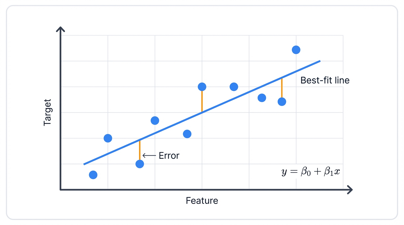
Linear regression finds the best straight line through your data points. Simple as that. You feed it input variables (features) and one continuous output variable (target), and the algorithm discovers the linear relationship connecting them.
What makes a line "best"? It minimizes the sum of squared distances between actual data points and the line itself. These distances? We call them residuals. Or errors. Squaring them heavily penalizes large errors and prevents positive and negative errors from canceling out—a technique called Ordinary Least Squares (OLS).
Picture this scenario: You have a scatter plot with house size on the x-axis and price on the y-axis, each dot representing a house that sold in your neighborhood. Linear regression draws the single straight line that best fits through this cloud of points, systematically minimizing the squared distances from points to the line. Use this line to predict any new house's price based on its size.
See Linear Regression in Action
This real-world example shows how linear regression learns to predict house prices from square footage. Watch the algorithm discover patterns in actual data.
import numpy as np
import matplotlib.pyplot as plt
from sklearn.linear_model import LinearRegression
from sklearn.metrics import mean_squared_error, r2_score
import pandas as pd

# Generate realistic house price data
np.random.seed(42)
n_houses = 100

# House sizes between 800 and 3000 square feet
house_sizes = np.random.uniform(800, 3000, n_houses)

# Price = base price + price per sqft + noise
# Realistic: $50k base + $120 per sqft + random variation
base_price = 50000
price_per_sqft = 120
noise = np.random.normal(0, 15000, n_houses) # $15k standard deviation
house_prices = base_price + price_per_sqft * house_sizes + noise

# Reshape for sklearn (needs 2D array)
X = house_sizes.reshape(-1, 1)
y = house_prices

print("Linear Regression: House Price Prediction")
print("=" * 45)
print(f"Dataset: {n_houses} houses")
print(f"Size range: {house_sizes.min():.0f} - {house_sizes.max():.0f} sqft")
print(f"Price range: ${house_prices.min():,.0f} - ${house_prices.max():,.0f}")

# Train linear regression model
model = LinearRegression()
model.fit(X, y)

# Get model parameters
intercept = model.intercept_
slope = model.coef_[0]

print(f"\nLearned Parameters:")
print(f"Intercept (β₀): ${intercept:,.0f}")
print(f"Slope (β₁): ${slope:.2f} per sqft")
print(f"\nModel Equation: Price = ${intercept:,.0f} + ${slope:.2f} × Size")

# Compare with true parameters
print(f"\nTrue vs Learned:")
print(f"True base price: ${base_price:,.0f}")
print(f"Learned intercept: ${intercept:,.0f}")
print(f"True price/sqft: ${price_per_sqft:.2f}")
print(f"Learned slope: ${slope:.2f}")

# Make predictions
y_pred = model.predict(X)

# Calculate metrics
mse = mean_squared_error(y, y_pred)
rmse = np.sqrt(mse)
r2 = r2_score(y, y_pred)

print(f"\nModel Performance:")
print(f"RMSE: ${rmse:,.0f}")
print(f"R² Score: {r2:.3f}")
print(f"Explanation: Model explains {r2*100:.1f}% of price variance")

# Example predictions
test_sizes = np.array([1000, 1500, 2000, 2500])
test_predictions = model.predict(test_sizes.reshape(-1, 1))

print(f"\nExample Predictions:")
for size, price in zip(test_sizes, test_predictions):
    print(f"{size:,} sqft → ${price:,.0f}")
This demonstrates the core linear regression workflow. Data in. Model learns. Predictions out. The beauty lies in its simplicity—once trained, predictions are just a multiplication and addition away.
The Mathematical Foundation
The equation is elegantly simple:
$$ \hat{y} = \beta_0 + \beta_1 x_1 + \beta_2 x_2 + \cdots + \beta_n x_n $$
Where:
- $\hat{y}$ is your predicted value
- $\beta_0$ is the intercept (baseline when all features are zero)
- $\beta_1, \beta_2, \ldots, \beta_n$ are coefficients (weights) for each feature
- $x_1, x_2, \ldots, x_n$ are your input features
Training? That's about finding the perfect $\beta$ values. The ones that minimize prediction error across all your training data.
Finding the Best Fit: Two Approaches
Method 1: The Normal Equation (Closed-Form Solution)
No iteration needed. Just solve directly. One calculation gives you the optimal coefficients—mathematically guaranteed to be the best possible solution for your data.
$$ \boldsymbol{\beta} = (\mathbf{X}^T \mathbf{X})^{-1} \mathbf{X}^T \mathbf{y} $$
Where $\mathbf{X}$ is your feature matrix (all your input data), $\mathbf{y}$ is your target vector (what you're predicting), and $^T$ means transpose. Looks complicated? It's actually elegant—a single matrix operation that computes the best-fit line.
- Advantage: Exact solution. No hyperparameters to tune. No convergence issues to worry about.
- Disadvantage: Computationally expensive for large feature sets. That matrix inversion? Costly when you have thousands of features.
Method 2: Gradient Descent (Iterative Optimization)
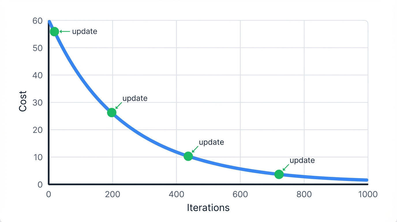
Start with random coefficients. Calculate error. Adjust coefficients to reduce error. Repeat until you can't improve anymore—a process that systematically walks downhill on the error landscape until reaching the bottom.
The update rule at iteration $t$ is:
$$ \beta_j^{(t+1)} = \beta_j^{(t)} - \alpha \frac{1}{m} \sum_{i=1}^{m} (h_{\beta}(x^{(i)}) - y^{(i)}) x_j^{(i)} $$
Where:
- $\alpha$ is the learning rate (step size)—too small and training crawls, too large and it explodes
- $m$ is number of training examples
- $h_{\beta}(x^{(i)})$ is the prediction for example $i$
- Advantage: Scales to massive datasets. Works when features number in the millions.
- Disadvantage: Requires tuning learning rate. May need many iterations. Never truly "finishes"—just gets close enough.
Gradient Descent Implementation
import numpy as np
import matplotlib.pyplot as plt
from sklearn.datasets import make_regression
from sklearn.preprocessing import StandardScaler

class LinearRegressionGD:
    def __init__(self, learning_rate=0.01, max_iterations=1000, tolerance=1e-6):
        self.learning_rate = learning_rate
        self.max_iterations = max_iterations
        self.tolerance = tolerance
        self.weights = None
        self.cost_history = []

    def compute_cost(self, X, y, weights):
        m = len(y)
        predictions = X @ weights
        cost = (1 / (2 * m)) * np.sum((predictions - y) ** 2)
        return cost

    def fit(self, X, y):
        # Add bias term
        m, n = X.shape
        X_with_bias = np.column_stack([np.ones(m), X])

        # Initialize weights
        self.weights = np.zeros(n + 1)

        # Gradient descent
        for i in range(self.max_iterations):
            # Compute predictions
            predictions = X_with_bias @ self.weights

            # Compute gradients
            gradient = (1 / m) * X_with_bias.T @ (predictions - y)

            # Update weights
            self.weights = self.weights - self.learning_rate * gradient

            # Track cost
            cost = self.compute_cost(X_with_bias, y, self.weights)
            self.cost_history.append(cost)

            # Check convergence
            if i > 0 and abs(self.cost_history[-2] - cost) < self.tolerance:
                print(f"Converged after {i+1} iterations")
                break

    def predict(self, X):
        m = X.shape[0]
        X_with_bias = np.column_stack([np.ones(m), X])
        return X_with_bias @ self.weights

# Demonstrate gradient descent
print("Gradient Descent: Training Process")
print("=" * 40)

# Generate synthetic dataset
X, y = make_regression(n_samples=100, n_features=1, noise=10, random_state=42)

# Scale features for better convergence
scaler = StandardScaler()
X_scaled = scaler.fit_transform(X)

# Train with different learning rates
learning_rates = [0.001, 0.01, 0.1]

for lr in learning_rates:
    model = LinearRegressionGD(learning_rate=lr, max_iterations=1000)
    model.fit(X_scaled, y)

    print(f"\nLearning Rate: {lr}")
    print(f"Iterations: {len(model.cost_history)}")
    print(f"Final Cost: {model.cost_history[-1]:.6f}")
    print(f"Weights: {model.weights}")
Key insights from gradient descent:
- Learning Rate is Critical: Too small means slow convergence; too large means overshooting or divergence.
- Feature Scaling Matters: Standardizing features (zero mean, unit variance) dramatically improves convergence.
- Cost Decreases Monotonically: Each iteration reduces cost until convergence—if it doesn't, your learning rate is too high.
- Early Stopping: Monitor cost changes; stop when improvements become negligible.
Logistic Regression: From Lines to Probabilities
Now for the twist. Logistic regression? Not actually regression. It's classification in disguise. The name's misleading—historically it emerged from regression techniques, but make no mistake, it predicts categories, not continuous values.
The core idea: Transform linear regression's unbounded output into a probability between 0 and 1 using the sigmoid function, then use that probability to assign class labels.
The Sigmoid Function: Gateway to Probabilities
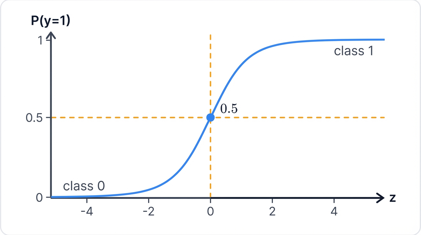
$$ \sigma(z) = \frac{1}{1 + e^{-z}} $$
Feed any number in. Get a probability out. Always between 0 and 1. Always smooth and differentiable. Perfect for machine learning.
Here's how it works: Start with linear combination $z = \beta_0 + \beta_1 x_1 + \beta_2 x_2 + \cdots + \beta_n x_n$, then squash it through sigmoid to get probability $P(y=1|x) = \sigma(z)$—transforming an unbounded prediction into a well-behaved probability.
- When $z = 0$: $\sigma(z) = 0.5$ (neutral, right on the decision boundary)
- When $z \to \infty$: $\sigma(z) \to 1$ (very confident "yes")
- When $z \to -\infty$: $\sigma(z) \to 0$ (very confident "no")
Classification in Practice
You get probabilities. Convert them to decisions. Simple threshold at 0.5 works for balanced problems—if $P(y=1|x) \geq 0.5$, predict class 1; otherwise predict class 0.
But here's the power: You can adjust that threshold based on your needs. False positives expensive? Raise the threshold to 0.7. False negatives catastrophic? Lower it to 0.3. The probability gives you control over the prediction's confidence level.
Implementing Logistic Regression
import numpy as np
from sklearn.datasets import make_classification
import matplotlib.pyplot as plt

class LogisticRegressionScratch:
    def __init__(self, learning_rate=0.01, max_iterations=1000):
        self.learning_rate = learning_rate
        self.max_iterations = max_iterations
        self.weights = None
        self.cost_history = []

    def sigmoid(self, z):
        return 1 / (1 + np.exp(-z))

    def fit(self, X, y):
        m, n = X.shape
        # Add bias term
        X_with_bias = np.column_stack([np.ones(m), X])

        # Initialize weights
        self.weights = np.zeros(n + 1)

        # Gradient descent
        for i in range(self.max_iterations):
            # Compute predictions
            z = X_with_bias @ self.weights
            predictions = self.sigmoid(z)

            # Compute cost (log loss)
            epsilon = 1e-15
            predictions = np.clip(predictions, epsilon, 1 - epsilon)
            cost = -np.mean(y * np.log(predictions) + (1 - y) * np.log(1 - predictions))
            self.cost_history.append(cost)

            # Gradient calculation
            gradient = X_with_bias.T @ (predictions - y) / m

            # Update weights
            self.weights = self.weights - self.learning_rate * gradient

            # Check convergence
            if i > 0 and abs(self.cost_history[-2] - cost) < 1e-8:
                print(f"Converged after {i+1} iterations")
                break

    def predict_proba(self, X):
        X_with_bias = np.column_stack([np.ones(X.shape[0]), X])
        return self.sigmoid(X_with_bias @ self.weights)

    def predict(self, X, threshold=0.5):
        return (self.predict_proba(X) >= threshold).astype(int)

# Demonstrate logistic regression training
print("Logistic Regression: Training Process Visualization")
print("=" * 52)

# Generate binary classification dataset
X, y = make_classification(
    n_samples=300, n_features=2, n_redundant=0, n_informative=2,
    n_clusters_per_class=1, random_state=42
)

# Train our implementation
model = LogisticRegressionScratch(learning_rate=0.1, max_iterations=1000)
model.fit(X, y)

print(f"Final weights: {model.weights}")
print(f"Training iterations: {len(model.cost_history)}")
print(f"Final cost: {model.cost_history[-1]:.6f}")

# Compare with sklearn
from sklearn.linear_model import LogisticRegression
sklearn_model = LogisticRegression(fit_intercept=True, random_state=42)
sklearn_model.fit(X, y)

print(f"\nComparison with sklearn:")
our_weights = model.weights
sklearn_weights = np.concatenate([sklearn_model.intercept_, sklearn_model.coef_[0]])
print(f"Our weights: {our_weights}")
print(f"Sklearn weights: {sklearn_weights}")
print(f"Difference: {np.abs(our_weights - sklearn_weights)}")

# Test predictions
test_accuracy_ours = np.mean(model.predict(X) == y)
test_accuracy_sklearn = sklearn_model.score(X, y)
print(f"\nAccuracy comparison:")
print(f"Our implementation: {test_accuracy_ours:.3f}")
print(f"Sklearn: {test_accuracy_sklearn:.3f}")

# Show cost function decrease
print(f"\nCost function progress:")
print(f"Initial cost: {model.cost_history[0]:.6f}")
print(f"Final cost: {model.cost_history[-1]:.6f}")
print(f"Cost reduction: {model.cost_history[0] - model.cost_history[-1]:.6f}")
Key insights from the training process:
- Sigmoid Function: Converts any real number to probability [0,1]
- Log Loss: Penalizes confident wrong predictions heavily
- Gradient Descent: Iteratively adjusts weights to minimize cost
- Convergence: Cost function decreases until weights stabilize
- No Analytical Solution: Unlike linear regression, requires optimization
Maximum Likelihood Intuition
MLE finds weights that make the observed data most likely:

Given data: [(x₁,y₁), (x₂,y₂), ..., (xₘ,yₘ)]

For each point (xᵢ,yᵢ):
If yᵢ = 1  We want P(y=1|xᵢ) to be high
If yᵢ = 0  We want P(y=0|xᵢ) = 1-P(y=1|xᵢ) to be high

Likelihood = ∏ᵢ P(yᵢ|xᵢ)

We find weights β that maximize this likelihood.
Gradient Descent Optimization
Since there's no direct solution, you optimize iteratively. Same process as linear regression—initialize weights, compute gradient, update weights, repeat—but with the logistic cost function steering the way.
The gradient has an elegant form:
$$ \frac{\partial}{\partial \beta_j} J(\boldsymbol{\beta}) = \frac{1}{m} \sum_{i=1}^{m} (h(\mathbf{x}_i) - y_i) x_{ij} $$
Notice how similar this looks to linear regression? Same mathematical structure. The update rule:
βⱼ := βⱼ - α(1/m)∑ᵢ₌₁ᵐ(h(xᵢ) - yᵢ)xᵢⱼ
The striking similarity of gradient descent update rules for both models—essentially (prediction - actual) × feature—isn't coincidence at all. It stems from deep mathematical property shared by broader model class: Generalized Linear Models (GLMs). Linear Regression (Normal distribution + identity link function) and Logistic Regression (Bernoulli distribution + logit link function) are GLM special cases, and this underlying unity explains why their learning dynamics are fundamentally similar and why techniques like regularization apply consistently to both.
The two training methods for linear regression represent a critical trade-off between analytical precision and iterative scalability, and understanding this trade-off shapes how we approach modern machine learning problems. The Normal Equation provides an exact, parameter-free solution but becomes computationally expensive for high-dimensional data due to the matrix inversion step (O(n_features³) complexity). Gradient Descent, with per-iteration complexity O(n_samples × n_features), is an approximate method that scales far better to the large, high-dimensional datasets common in modern ML. This shift from analytical to iterative methods was a necessary "Big Data" era adaptation, but it introduced new challenges: tuning the learning rate and the critical need for feature scaling to ensure stable convergence.
Understanding the Key Parameters
Model parameters divide into two categories. Learn this distinction. Those learned from data and those you specify before training—each plays a fundamentally different role in how your model behaves.
Model Parameters (Learned) represent the values that algorithms discover during training, forming the core of the learned function that makes predictions on new data, and these are what the model "knows" after seeing your examples. Coefficients or Weights (β₁,...,βₙ or w₁,...,wₙ) quantify the precise relationship between each input feature and the target variable, indicating both the direction and magnitude of each feature's influence on the final prediction. The Intercept or Bias Term (β₀ or b) provides the baseline prediction value when all features equal zero, establishing the starting point for the linear combination that generates predictions.
Hyperparameters (You Set These)
These aren't learned from data. You configure them to control the learning process. They dramatically affect performance.
- Regularization Strength (α, λ, or C) Controls the penalty on coefficients to prevent overfitting. Higher α/λ (or lower C) means stronger regularization.
- Regularization Type L1 (Lasso), L2 (Ridge), or Elastic Net (combination)
- Learning Rate (α or η) Step size for gradient descent. Critical for convergence.
- Solver The optimization algorithm ('lbfgs', 'liblinear', 'sag'). Different solvers work better for different dataset sizes.
Practical Implementation: Making It Work in the Real World
Theory's nice. But let's talk reality. You need to understand data requirements, computational costs, and tools that actually work in production environments.
Data Requirements: What Your Models Need to Succeed
Your data makes or breaks these models. No amount of hyperparameter tuning saves you from bad data. Here's what matters:
Data Types
Linear Regression requires continuous numerical targets such as house prices, temperatures, or sales figures that can take any value within a reasonable range, making it perfect for "how much" or "how many" questions. Logistic Regression requires categorical targets such as spam/not spam decisions or yes/no classifications that represent discrete outcomes rather than continuous values, making it ideal for "which category" or "yes or no" questions. Features for both algorithms work well with numerical inputs, though categorical features require proper encoding techniques like one-hot encoding before algorithms can process them effectively.
Data Preprocessing
Raw data is messy. Always. Here's what you need to fix:
Missing Values cannot be handled natively by these algorithms, requiring either row deletion (wasteful if data is scarce) or imputation using statistical methods like mean, median, or more sophisticated model-based approaches before training can proceed. Outliers present significant risks since extreme values can dramatically shift entire models away from true underlying patterns, requiring identification and removal or transformation techniques like robust scaling or winsorization. Feature Scaling proves essential for gradient descent convergence and regularization effectiveness, typically through standardization (zero mean, unit variance) or normalization (0-1 range) to prevent features with larger scales from dominating the optimization process. Categorical Encoding converts text-based categories into numerical representations that algorithms can process, with one-hot encoding creating binary columns for each category while avoiding artificial ordering assumptions that could mislead the learning process.
Dataset Sizes
- Small to Medium (<100K samples) Both models shine here
- Logistic Regression Rule Need at least 10 examples of your rarest class per feature for stable estimates
- Large Datasets (>1M samples) Use Stochastic Gradient Descent (SGD) with mini-batches for scalability
Computational Complexity: Speed Matters in Production
Speed matters in production. Real systems need real-time responses. Your computational cost depends on the algorithm, sample count (m), and feature count (n).
Training Complexity
- Normal Equation O(n³) dominated by matrix inversion. Fast for n<1,000, impossible for large feature sets.
- Batch Gradient Descent O(k×m×n) where k is iterations. Scales with features but slow for massive datasets.
- SGD O(k×n) per iteration. Uses one sample at a time. Faster on huge datasets despite more iterations.
Prediction Complexity
O(n) per prediction—just a dot product. Blazing fast for real-time applications. This is why these models dominate production environments where millisecond response times matter.
Normal Equation hits wall with feature count. Perfect for narrow datasets (hundreds of features), but modern wide datasets (genomics with tens of thousands of genes, text analysis with hundreds of thousands of words) make O(n³) cost prohibitive, forcing you into iterative methods like gradient descent and changing entire workflow.
| Training Method | Training Time Complexity | Prediction Time Complexity | Space Complexity | Key Advantage | Key Disadvantage |
|---|---|---|---|---|---|
| Normal Equation | O(n³ + mn²) | O(n) | O(n²) | Exact, no hyperparameters to tune | Infeasible for large number of features (n) |
| Batch Gradient Descent | O(k⋅m⋅n) | O(n) | O(mn) | Guaranteed to converge to global minimum (for convex problems) | Slow on very large number of samples (m) |
| Stochastic Gradient Descent | O(k⋅n) (approx.) | O(n) | O(mn) | Highly scalable for large m, allows online learning | Noisy updates, may not converge to exact minimum |
Note: m = number of samples, n = number of features, k = number of iterations.
Popular Libraries and Frameworks: Your Toolkit
The ecosystem makes implementation straightforward. Here's what actually works in production:
Python Ecosystem
- Scikit-learn The gold standard. Optimized implementations of `LinearRegression` and `LogisticRegression` plus the full ML pipeline toolkit—preprocessing, cross-validation, metrics, everything.
- Statsmodels For when you need rigorous statistics - p-values, confidence intervals, diagnostic tests. Academic research loves this.
- Core Libraries NumPy (numerical computation), Pandas (data wrangling), Matplotlib/Seaborn (visualization). The foundation of everything.
Other Options
- LIBLINEAR Highly efficient C++ library for large-scale classification. Powers Scikit-learn's 'liblinear' solver.
- R Built-in `lm()` and `glm()` functions. Standard in academic statistics.
The Great Divide: Scikit-learn vs Statsmodels reflects different goals, and choosing between them reveals your mission. Scikit-learn optimizes for prediction - fit/predict workflows, pipelines, cross-validation, everything designed for building accurate models. Statsmodels is built for inference - hypothesis testing, parameter interpretation, rich summaries, everything designed for understanding relationships. Your choice reveals your mission: prediction accuracy (ML) or causal understanding (statistics).
Problem-Solving Capabilities: Where These Models Excel
These models tackle diverse problems across industries. Success depends on matching model capabilities to your problem type.
Primary Use Cases and Output Types
Linear Regression
- Purpose Predicting continuous values ("How much?", "How many?")
- Output Single numerical prediction ($350,000, 25.5°C). Coefficients are directly interpretable - a coefficient of 50 for "square_feet" means each additional square foot adds $50 to the price.
Logistic Regression
- Purpose Binary or multiclass classification ("Will this customer churn?", "Which product category?")
- Output Probabilities (0-1) that you convert to class labels using a threshold (usually 0.5). A 0.85 probability becomes "Yes, churn."
- Interpretation Coefficients show how log-odds change per unit increase in a feature. Convert to odds ratios for easier understanding.
Real-World Applications: Where You'll Use These Models
These are workhorses across industries thanks to speed and interpretability. Let's see them in action.
Linear Regression Applications
Business & Finance
- Sales forecasting (advertising spend, seasonality, economic indicators)
- Real estate valuation (size, rooms, location)
- Risk assessment and asset pricing (CAPM models)
Healthcare & Agriculture
- Medical research (blood pressure vs. drug dosage)
- Crop yield prediction (fertilizer, water, sunlight)
Sports Analytics
- Player performance modeling (training, age, physical attributes)
Logistic Regression Applications
Healthcare
- Disease prediction (heart disease, diabetes from clinical data)
- Tumor classification (malignant vs. benign from imaging)
Finance & Banking
- Credit scoring and loan approval (default risk assessment)
- Fraud detection (transaction pattern analysis)
Marketing & E-commerce
- Customer churn prediction (subscription cancellation likelihood)
- Click-through rate estimation (ad performance)
- Spam detection (email classification)
Performance Characteristics
Performance hinges on your data's structure. Here's when they shine and when they struggle:
When They Excel
- Linear relationships Features relate linearly to target (or log-odds for logistic)
- Low multicollinearity Features aren't highly correlated with each other
- Clean data Proper preprocessing, outliers handled, features scaled
- Strong signal Clear patterns outweigh random noise
When They Struggle
- Non-linear relationships Can't capture U-shapes, curves, or complex patterns
- Feature interactions Won't automatically detect when one feature's effect depends on another
- High dimensionality Many irrelevant features cause overfitting (need regularization)
- Outliers Extreme values skew the entire model
Real-World Application: Customer Churn Prediction
import pandas as pd
import numpy as np
from sklearn.model_selection import train_test_split, cross_val_score
from sklearn.linear_model import LogisticRegression
from sklearn.preprocessing import StandardScaler, LabelEncoder
from sklearn.metrics import classification_report, roc_auc_score
from sklearn.pipeline import Pipeline

# Create realistic customer churn dataset
np.random.seed(42)
n_customers = 1000

# Generate customer features
data = {
    'tenure_months': np.random.exponential(24, n_customers),
    'monthly_spend': np.random.lognormal(4, 0.5, n_customers),
    'support_tickets': np.random.poisson(2, n_customers),
    'contract_type': np.random.choice(['month', 'annual', '2-year'], n_customers, p=[0.5, 0.3, 0.2]),
    'age': np.random.normal(45, 15, n_customers),
    'satisfaction_score': np.random.beta(7, 3, n_customers) * 5 # 0-5 scale, skewed toward higher scores
}

# Create realistic churn probability based on features
churn_logits = (
    -2.0 + # Base rate (low churn)
    -0.05 * data['tenure_months'] + # Longer tenure = less churn
    -0.0005 * data['monthly_spend'] + # Higher spend = less churn
    0.3 * data['support_tickets'] + # More tickets = more churn
    -0.5 * (data['contract_type'] == '2-year').astype(int) + # Long contracts = less churn
    -0.02 * data['age'] + # Older customers = less churn
    -0.8 * data['satisfaction_score'] # Higher satisfaction = less churn
)

churn_probabilities = 1 / (1 + np.exp(-churn_logits))
data['churned'] = np.random.binomial(1, churn_probabilities, n_customers)

# Convert to DataFrame
df = pd.DataFrame(data)

print("Customer Churn Prediction with Logistic Regression")
print("=" * 52)
print(f"Dataset: {len(df)} customers")
print(f"Churn rate: {df['churned'].mean():.1%}")
print(f"\nFeature Statistics:")
print(df.describe())

# Prepare features
# Encode categorical variables
le = LabelEncoder()
df['contract_encoded'] = le.fit_transform(df['contract_type'])

# Select features for modeling
features = ['tenure_months', 'monthly_spend', 'support_tickets',
           'contract_encoded', 'age', 'satisfaction_score']
X = df[features]
y = df['churned']

# Split data
X_train, X_test, y_train, y_test = train_test_split(
    X, y, test_size=0.2, random_state=42, stratify=y
)

# Create and train model with pipeline
pipeline = Pipeline([
    ('scaler', StandardScaler()),
    ('classifier', LogisticRegression(random_state=42))
])

pipeline.fit(X_train, y_train)

# Make predictions
y_pred = pipeline.predict(X_test)
y_pred_proba = pipeline.predict_proba(X_test)[:, 1]

# Evaluate model
auc_score = roc_auc_score(y_test, y_pred_proba)
print(f"\nModel Performance:")
print(f"AUC Score: {auc_score:.3f}")
print(f"\nDetailed Classification Report:")
print(classification_report(y_test, y_pred, target_names=['Retained', 'Churned']))

# Feature importance (coefficients)
coefficients = pipeline.named_steps['classifier'].coef_[0]
feature_importance = pd.DataFrame({
    'feature': features,
    'coefficient': coefficients,
    'abs_coefficient': np.abs(coefficients)
}).sort_values('abs_coefficient', ascending=False)

print("\nFeature Importance (by coefficient magnitude):")
print(feature_importance)

# Interpret coefficients
print("\nCoefficient Interpretation:")
for idx, row in feature_importance.iterrows():
    feature = row['feature']
    coef = row['coefficient']
    if coef > 0:
        print(f"{feature}: Increases churn probability (coef={coef:.4f})")
    else:
        print(f"{feature}: Decreases churn probability (coef={coef:.4f})")
This example demonstrates the complete workflow: data generation, preprocessing, model training, evaluation, and interpretation—everything you need for real-world deployment.
Advanced Techniques: Taking It Further
Regularization: Preventing Overfitting
Regularization adds a penalty term to the cost function. Why? To discourage large coefficients that might fit training noise instead of true patterns.
L2 Regularization (Ridge)
Adds penalty proportional to square of coefficients:
$$ J(\boldsymbol{\beta}) = \text{MSE}(\boldsymbol{\beta}) + \alpha \sum_{j=1}^{n} \beta_j^2 $$
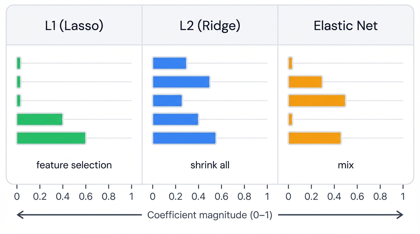
- Effect: Shrinks all coefficients toward zero but keeps them all
- Use When: All features potentially relevant
- Benefit: Handles multicollinearity well
L1 Regularization (Lasso)
Adds penalty proportional to absolute value of coefficients:
$$ J(\boldsymbol{\beta}) = \text{MSE}(\boldsymbol{\beta}) + \alpha \sum_{j=1}^{n} |\beta_j| $$
- Effect: Drives some coefficients exactly to zero (feature selection)
- Use When: Many irrelevant features expected
- Benefit: Automatic feature selection
Elastic Net (Best of Both)
Combines L1 and L2 penalties:
$$ J(\boldsymbol{\beta}) = \text{MSE}(\boldsymbol{\beta}) + \alpha_1 \sum_{j=1}^{n} |\beta_j| + \alpha_2 \sum_{j=1}^{n} \beta_j^2 $$
- Effect: Balances feature selection (L1) with coefficient shrinkage (L2)
- Use When: Correlated features and need feature selection
- Benefit: More stable than pure L1, more selective than pure L2
Regularization in Practice
import numpy as np
from sklearn.datasets import make_regression
from sklearn.linear_model import Ridge, Lasso, ElasticNet, LinearRegression
from sklearn.model_selection import train_test_split
from sklearn.metrics import mean_squared_error, r2_score
import matplotlib.pyplot as plt

# Generate dataset with some irrelevant features
X, y, true_coef = make_regression(
    n_samples=100, n_features=20, n_informative=10,
    noise=10, coef=True, random_state=42
)

X_train, X_test, y_train, y_test = train_test_split(
    X, y, test_size=0.3, random_state=42
)

print("Regularization Comparison: Ridge vs Lasso vs Elastic Net")
print("=" * 60)

# Train models
models = {
    'Linear Regression': LinearRegression(),
    'Ridge (L2)': Ridge(alpha=1.0),
    'Lasso (L1)': Lasso(alpha=1.0),
    'Elastic Net': ElasticNet(alpha=1.0, l1_ratio=0.5)
}

results = []

for name, model in models.items():
    # Train
    model.fit(X_train, y_train)

    # Predict
    y_pred_train = model.predict(X_train)
    y_pred_test = model.predict(X_test)

    # Evaluate
    train_mse = mean_squared_error(y_train, y_pred_train)
    test_mse = mean_squared_error(y_test, y_pred_test)
    train_r2 = r2_score(y_train, y_pred_train)
    test_r2 = r2_score(y_test, y_pred_test)

    # Count non-zero coefficients
    if hasattr(model, 'coef_'):
        n_nonzero = np.sum(np.abs(model.coef_) > 1e-5)
    else:
        n_nonzero = len(model.coef_)

    results.append({
        'Model': name,
        'Train MSE': train_mse,
        'Test MSE': test_mse,
        'Train R²': train_r2,
        'Test R²': test_r2,
        'Non-zero Coefs': n_nonzero
    })

    print(f"\n{name}:")
    print(f"  Train MSE: {train_mse:.2f}, Test MSE: {test_mse:.2f}")
    print(f"  Train R²: {train_r2:.3f}, Test R²: {test_r2:.3f}")
    print(f"  Non-zero coefficients: {n_nonzero}/20")
    print(f"  Overfitting gap: {train_r2 - test_r2:.3f}")

# Compare with true coefficients
print(f"\nTrue informative features: 10")
print(f"True zero coefficients: 10")
print(f"\nLasso correctly identified {np.sum(models['Lasso (L1)'].coef_ == 0)} zero coefficients")
Key takeaways:
- Ridge: Shrinks all coefficients, reduces overfitting without feature selection
- Lasso: Performs automatic feature selection by zeroing coefficients
- Elastic Net: Combines benefits of both, more stable when features correlate
- Alpha Parameter: Controls regularization strength—higher means more penalty
Polynomial Features: Capturing Non-Linearity
Linear models can capture non-linear relationships. How? Transform your features. Add polynomial terms and interaction terms to capture curves and feature combinations.
import numpy as np
from sklearn.preprocessing import PolynomialFeatures
from sklearn.linear_model import LinearRegression
from sklearn.pipeline import Pipeline
import matplotlib.pyplot as plt

# Generate non-linear data
np.random.seed(42)
X = np.sort(5 * np.random.rand(100, 1), axis=0)
y = np.sin(X).ravel() + np.random.normal(0, 0.1, X.shape[0])

print("Polynomial Regression: Capturing Non-Linear Patterns")
print("=" * 52)

# Test different polynomial degrees
degrees = [1, 2, 3, 5, 10]

for degree in degrees:
    # Create pipeline
    model = Pipeline([
        ('poly', PolynomialFeatures(degree=degree)),
        ('linear', LinearRegression())
    ])

    # Fit
    model.fit(X, y)

    # Evaluate
    y_pred = model.predict(X)
    mse = mean_squared_error(y, y_pred)
    r2 = r2_score(y, y_pred)

    # Count features
    n_features = model.named_steps['poly'].n_output_features_

    print(f"\nDegree {degree}:")
    print(f"  Features created: {n_features}")
    print(f"  MSE: {mse:.4f}")
    print(f"  R²: {r2:.3f}")

    if degree <= 3:
        print(f"  Status: Good fit")
    elif degree <= 5:
        print(f"  Status: Potential overfitting")
    else:
        print(f"  Status: Likely overfitting")

print("\nKey Insight:")
print("Higher degree polynomials fit training data better but may overfit.")
print("Use cross-validation to find optimal degree.")
Polynomial features let linear models capture curves. Degree 2 adds squares and interactions. Degree 3 adds cubes. But beware—high degrees overfit easily, fitting training noise instead of true patterns.
Model Evaluation and Validation
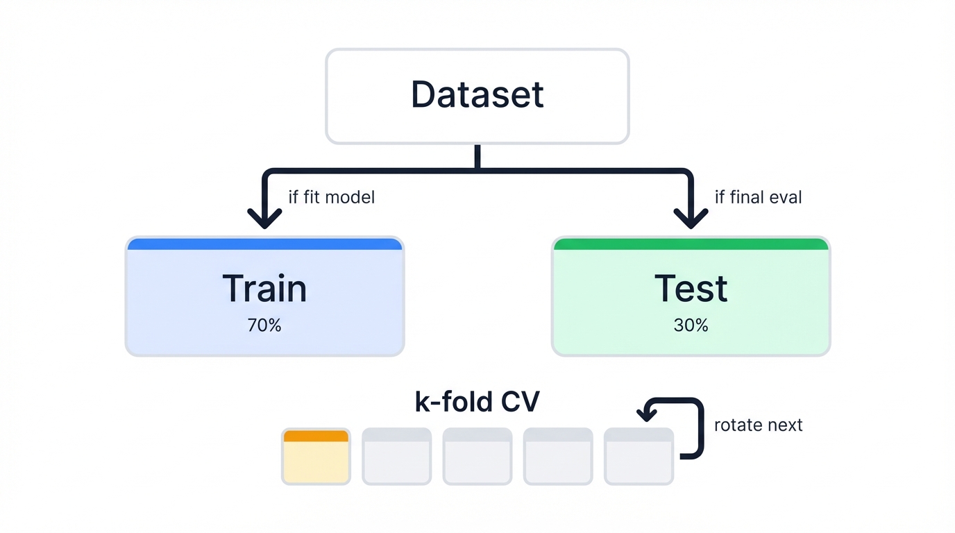
Train-Test Split: The Foundation
Never evaluate on training data. Ever. It's like grading a student's exam with questions they've already seen—meaningless performance assessment.
from sklearn.model_selection import train_test_split

# Standard 80-20 split
X_train, X_test, y_train, y_test = train_test_split(
    X, y, test_size=0.2, random_state=42
)

# For classification, use stratify to maintain class proportions
X_train, X_test, y_train, y_test = train_test_split(
    X, y, test_size=0.2, random_state=42, stratify=y
)
Best Practices
- Standard split: 80% train, 20% test
- Small datasets: 70-30 or even 60-40 split
- Large datasets: Can use 90-10 (more data for training)
- Always set random_state for reproducibility
- Stratify for classification to maintain class balance
Cross-Validation: More Reliable Estimates
Single train-test split is noisy. One bad split misleads you. Cross-validation averages over multiple splits—more reliable performance estimates.
from sklearn.model_selection import cross_val_score, KFold

# K-Fold Cross-Validation
model = LinearRegression()

# 5-fold CV
scores = cross_val_score(model, X, y, cv=5, scoring='r2')

print(f"Cross-Validation R² Scores: {scores}")
print(f"Mean R²: {scores.mean():.3f}")
print(f"Std R²: {scores.std():.3f}")

# For classification
log_model = LogisticRegression()
cv_scores = cross_val_score(log_model, X, y, cv=5, scoring='roc_auc')

print(f"\nCross-Validation AUC Scores: {cv_scores}")
print(f"Mean AUC: {cv_scores.mean():.3f}")
print(f"Std AUC: {cv_scores.std():.3f}")
K-fold CV splits data into K parts. Train on K-1 parts, test on remaining part. Repeat K times, each part serving as test set once. Average the K scores for final estimate—more robust than single split.
Best Practices Checklist
- Handle Missing Values: Impute before scaling to avoid errors
- Scale Numeric Features: Essential for regularization and gradient descent
- Encode Categories: One-hot encoding for nominal, label encoding for ordinal
- Split First: Prevent data leakage by splitting before preprocessing
- Pipeline Everything: Ensures same preprocessing on train/test/new data
- Handle Outliers: Consider robust scaling or outlier removal
- Feature Engineering: Create new features before preprocessing
- Check Assumptions After fitting, verify assumptions (residual plots for linear regression). Violated assumptions = unreliable inferences.
- Use Pipelines Chain preprocessing + model in Scikit-learn pipelines. Prevents data leakage, ensures reproducibility.
Common Pitfalls
- Ignoring Assumptions Skipping assumption checks leads to wrong conclusions, especially for inference.
- Misinterpreting Coefficients Don't treat logistic coefficients as direct probability effects. Don't ignore "holding all else constant." Don't assign causation to correlation.
- Forgetting Feature Scaling Unscaled features cause poor convergence and bias toward larger-scale features.
- Overfitting with Many Features Without regularization, more features always improve training performance but hurt generalization.
- Data Leakage Using test set info during training (e.g., fitting scalers on full dataset) gives false optimism.
Hyperparameter Tuning
Optimizing hyperparameters maximizes performance. Here's how to do it right.
- Cross-Validation Use k-fold CV for reliable performance estimates on unseen data.
- Grid/Random Search Systematically search optimal regularization strength (α or C) and L1 ratio (Elastic Net). Use GridSearchCV or RandomizedSearchCV.
- Specialized CV Models RidgeCV, LassoCV, LogisticRegressionCV have built-in efficient CV. Much faster than GridSearchCV.
Hyperparameter Tuning Best Practices
Best Practice: Following these recommended practices will help you achieve optimal results and avoid common pitfalls.
import numpy as np
from sklearn.datasets import make_classification
from sklearn.model_selection import GridSearchCV, RandomizedSearchCV, train_test_split
from sklearn.linear_model import LogisticRegression, LogisticRegressionCV
from sklearn.preprocessing import StandardScaler
from sklearn.pipeline import Pipeline
from sklearn.metrics import classification_report, roc_auc_score
import time

# Generate dataset
X, y = make_classification(
    n_samples=1000, n_features=20, n_informative=10,
    n_redundant=10, random_state=42
)

X_train, X_test, y_train, y_test = train_test_split(
    X, y, test_size=0.2, random_state=42, stratify=y
)

print("Hyperparameter Tuning: Grid Search vs Random Search vs CV Models")
print("=" * 68)
print(f"Dataset: {X.shape[0]} samples, {X.shape[1]} features")

# Method 1: Manual Grid Search
print(f"\n1. Grid Search (Exhaustive):")
start_time = time.time()

pipeline_grid = Pipeline([
    ('scaler', StandardScaler()),
    ('classifier', LogisticRegression(random_state=42, max_iter=1000))
])

param_grid = {
    'classifier__C': [0.01, 0.1, 1, 10, 100],
    'classifier__penalty': ['l1', 'l2', 'elasticnet'],
    'classifier__solver': ['liblinear', 'saga'],
    'classifier__l1_ratio': [0.15, 0.5, 0.85] # Only used for elasticnet
}

# Note: We'll filter incompatible combinations
grid_search = GridSearchCV(
    pipeline_grid, param_grid, cv=5, scoring='roc_auc',
    n_jobs=-1, verbose=0
)

# Filter parameter combinations to avoid solver compatibility issues
valid_params = []
for C in param_grid['classifier__C']:
    for penalty in param_grid['classifier__penalty']:
        for solver in param_grid['classifier__solver']:
            if penalty == 'l1' and solver not in ['liblinear', 'saga']:
                continue
            if penalty == 'elasticnet' and solver != 'saga':
                continue

            params = {
                'classifier__C': C,
                'classifier__penalty': penalty,
                'classifier__solver': solver
            }

            if penalty == 'elasticnet':
                for l1_ratio in param_grid['classifier__l1_ratio']:
                    params_copy = params.copy()
                    params_copy['classifier__l1_ratio'] = l1_ratio
                    valid_params.append(params_copy)
            else:
                valid_params.append(params)

print(f"  Parameter combinations to test: {len(valid_params)}")

# Simplified grid search with compatible parameters
simple_param_grid = {
    'classifier__C': [0.01, 0.1, 1, 10, 100],
    'classifier__penalty': ['l2'],
    'classifier__solver': ['lbfgs']
}

grid_search = GridSearchCV(
    pipeline_grid, simple_param_grid, cv=5, scoring='roc_auc', n_jobs=-1
)
grid_search.fit(X_train, y_train)

grid_time = time.time() - start_time
print(f"  Time taken: {grid_time:.2f} seconds")
print(f"  Best parameters: {grid_search.best_params_}")
print(f"  Best CV score: {grid_search.best_score_:.4f}")

# Method 2: Random Search
print(f"\n2. Random Search (Sampling):")
start_time = time.time()

from scipy.stats import uniform, loguniform

param_distributions = {
    'classifier__C': loguniform(0.01, 100),
    'classifier__penalty': ['l2'],
    'classifier__solver': ['lbfgs']
}

random_search = RandomizedSearchCV(
    pipeline_grid, param_distributions, n_iter=20, cv=5,
    scoring='roc_auc', n_jobs=-1, random_state=42
)
random_search.fit(X_train, y_train)

random_time = time.time() - start_time
print(f"  Time taken: {random_time:.2f} seconds")
print(f"  Best parameters: {random_search.best_params_}")
print(f"  Best CV score: {random_search.best_score_:.4f}")

# Method 3: Built-in CV (Most Efficient)
print(f"\n3. LogisticRegressionCV (Built-in):")
start_time = time.time()

scaler = StandardScaler()
X_train_scaled = scaler.fit_transform(X_train)
X_test_scaled = scaler.transform(X_test)

cv_model = LogisticRegressionCV(
    Cs=[0.01, 0.1, 1, 10, 100], # C values to try
    cv=5,
    scoring='roc_auc',
    random_state=42,
    max_iter=1000,
    n_jobs=-1
)
cv_model.fit(X_train_scaled, y_train)

cv_time = time.time() - start_time
print(f"  Time taken: {cv_time:.2f} seconds")
print(f"  Best C: {cv_model.C_[0]:.4f}")
print(f"  Best CV score: {cv_model.scores_[1].mean(axis=0).max():.4f}")

# Compare all methods on test set
print(f"\nTest Set Performance Comparison:")
print("-" * 40)

methods = [
    ('Grid Search', grid_search),
    ('Random Search', random_search),
    ('CV Model', cv_model)
]

for name, model in methods:
    if name == 'CV Model':
        y_pred = model.predict(X_test_scaled)
        y_pred_proba = model.predict_proba(X_test_scaled)[:, 1]
    else:
        y_pred = model.predict(X_test)
        y_pred_proba = model.predict_proba(X_test)[:, 1]

    auc = roc_auc_score(y_test, y_pred_proba)
    accuracy = (y_pred == y_test).mean()

    print(f"{name:15s}: AUC={auc:.4f}, Accuracy={accuracy:.4f}")

# Speed comparison
print(f"\nSpeed Comparison:")
print(f"Grid Search: {grid_time:.2f}s")
print(f"Random Search: {random_time:.2f}s")
print(f"CV Model: {cv_time:.2f}s")
print(f"\nSpeedup vs Grid Search:")
print(f"Random Search: {grid_time/random_time:.1f}x faster")
print(f"CV Model: {grid_time/cv_time:.1f}x faster")

# Best practices summary
print(f"\n" + "="*50)
print("Hyperparameter Tuning Best Practices")
print("="*50)
print("1. Use built-in CV models when available (LogisticRegressionCV, RidgeCV, LassoCV)")
print("2. Random search for initial exploration, grid search for final tuning")
print("3. Always use separate validation set or cross-validation")
print("4. Start with wide range, then narrow down")
print("5. Consider computational budget vs. performance gains")
print("6. Monitor for overfitting (validation score << training score)")
Hyperparameter Tuning Decision Tree
Hyperparameter Tuning Strategy:

┌─ Small dataset (<1000 samples)?
│ ├─ Yes → Use GridSearchCV (can afford exhaustive search)
│ └─ No → Continue below
│
├─ Many hyperparameters (>3)?
│ ├─ Yes → Use RandomizedSearchCV first, then GridSearch on best region
│ └─ No → Continue below
│
├─ Using standard algorithms (Ridge, Lasso, LogisticRegression)?
│ ├─ Yes → Use built-in CV models (RidgeCV, LassoCV, LogisticRegressionCV)
│ └─ No → Use RandomizedSearchCV
│
└─ Limited time/compute?
  ├─ Yes → Use built-in CV or RandomizedSearchCV with low n_iter
  └─ No → Use GridSearchCV for optimal results

Hyperparameter Ranges:
├─ C (LogisticRegression): [0.01, 0.1, 1, 10, 100]
├─ alpha (Ridge/Lasso): [0.01, 0.1, 1, 10, 100]
├─ l1_ratio (ElasticNet): [0.1, 0.3, 0.5, 0.7, 0.9]
└─ max_iter: [1000, 5000] (increase if convergence issues)
Evaluation Metrics
Choosing the right metric is critical for assessing goal achievement. Wrong metric? Wrong conclusions.
For Linear Regression
- MSE Average squared differences. What OLS minimizes. Sensitive to outliers due to squaring.
- RMSE √MSE. Same units as target, more interpretable.
- MAE Average absolute differences. Less sensitive to outliers than MSE.
- R² Proportion of variance explained by predictors (0-1, higher better). Misleading because it always increases with more variables. Use Adjusted R² for multiple regression.
For Logistic Regression
- Accuracy Correctly classified proportion. Misleading on imbalanced datasets.
- Confusion Matrix Table showing TP, TN, FP, FN performance breakdown.
- Precision TP/(TP+FP). Matters when false positives are costly.
- Recall TP/(TP+FN). Matters when false negatives are costly (medical diagnosis).
- F1-Score Harmonic mean of precision and recall. Single balanced metric.
- AUC-ROC Area under ROC curve. Measures class separation ability across thresholds (1.0 = perfect, 0.5 = random).
Recent Developments: Old Dogs, New Tricks
These are among the oldest ML models. Ancient by tech standards. Yet research continues refining their application and integrating them into modern AI pipelines.
Current Research
Recent work (2023-2024) focuses less on new variants, more on understanding nuanced behavior in modern optimization and overparameterized settings—exploring edge cases where classical theory breaks down.
Optimization Dynamics: Research explores gradient descent with large, adaptive step sizes, and the findings challenge everything we thought we knew about convergence. For linearly separable data, step sizes violating classical convergence criteria can actually converge faster—counterintuitive but true. This "Edge-of-Stability" regime challenges traditional wisdom and explains aggressive learning rates' effectiveness in deep learning. Very large step sizes can reduce GD for logistic regression to batch Perceptron.
Overparameterization: Classical stats warns against more parameters than data points—a cardinal sin in traditional statistics. But deep learning shows heavily overparameterized models can generalize well, contradicting decades of statistical wisdom. Recent work explores "benign overfitting" in linear/GLMs, showing that even simple overparameterized models can predict well and be theoretically justified—2024 research finally explains this puzzling phenomenon.
Interpretability & XAI: Pushback against "linear models are inherently interpretable"—a comfortable myth finally being challenged. Multicollinearity, feature transforms, and local vs. global effects mean simple models need rigorous XAI techniques (SHAP, LIME) just like black boxes to avoid misleading interpretations.
Fairness in GLMs: Algorithmic fairness is critical in deployed systems affecting people's lives. New methods ensure fairness via convex penalty terms, enabling efficient optimization while mitigating bias.
Future Directions
LLM Integration: Surprising research shows pre-trained LLMs can perform regression through in-context learning without gradient training—no fine-tuning needed. 2024 studies show GPT-4 and Claude 3 rival Random Forest performance just from prompted examples. Future: generalist AI models handling foundational statistical tasks.
Automated Feature Engineering: Models are old but data is increasingly complex—high-dimensional, messy, full of hidden patterns. Future development will integrate automated tools generating polynomial features, interactions, and transformations to help linear models capture non-linearities.
Advanced GLMs: Continuing GLM framework extensions for complex data structures—Negative Binomial for over-dispersed counts, Beta-Binomial for proportional data with litter effects.
Industry Trends
Despite complex algorithm proliferation, these models remain highly relevant and widely used. Why? Speed. Interpretability. Reliability.
The Universal Baseline: Starting point for any regression/classification task. Speed and simplicity perfect for quick baseline establishment against which complex models must be compared—if your neural network can't beat logistic regression, you've got problems.
Production in Regulated Industries: Finance, healthcare, insurance often require highly interpretable models due to regulations/business needs—"the model says you're high risk" doesn't fly without explanation. Well-tuned linear/logistic models preferred over black boxes, even with slight accuracy trade-offs.
Causal Analysis: Goal isn't just prediction but understanding outcome drivers—why things happen, not just what will happen. Primary tools for explanatory modeling answering "How much does marketing spend impact sales?"
Components of Complex Systems: Used within larger systems, often in surprising ways. Deep network final layers are typically softmax (multinomial logistic). Used in ensemble stacking where complex model predictions feed into final simple linear model.
Learning Resources: Your Next Steps
To deepen your understanding, abundant high-quality resources exist. From seminal papers to interactive courses and code repositories. Here's your roadmap.
Essential Papers
- Legendre (1805) First published account of least squares - mathematical foundation of linear regression
- Verhulst (1838) Introduced logistic function for population growth - later became core of logistic regression
- Cox (1958) Landmark paper formalizing logistic regression for binary classification
- Nelder & Wedderburn (1972) Introduced GLM framework unifying linear/logistic regression and many other models
- Tripepi et al. (2008) Practical overview of application and interpretation in medical research
Tutorials and Courses
- Google ML Crash Course Fast-paced, practical introduction with interactive modules on both regression types. Covers loss functions and gradient descent.
- Andrew Ng's ML Course (Coursera/Stanford) Most popular foundational course. Early weeks provide intuitive yet rigorous introduction including gradient descent derivations.
- Scikit-learn User Guide Comprehensive guide to linear models with mathematical formulations, solvers, and practical tips.
- Statsmodels Documentation For statistical inference focus - detailed examples of model fitting and result interpretation.
Code Examples
Hands-on implementation is crucial for mastering these algorithms. Reading isn't enough. You must code.
- GitHub Topic linear-regression-python: Curated repositories implementing linear regression, showcasing use cases from housing prices to student grades.
- Linear Regression from Scratch Clear Python implementation with custom MSE and gradient descent functions. Excellent educational tool.
- Kaggle Notebooks Thousands of examples applying models to real datasets with detailed EDA and feature engineering. Search "Linear Regression Benchmark" or "Logistic Regression Tutorial."
- Scikit-learn Examples Gallery of plots and code demonstrating various features, solver comparisons, and regularization techniques.
Benchmark Datasets
For Regression:
- Boston Housing Classic median house value prediction
- Diabetes Disease progression prediction
- UCI Repository "Wine Quality," "Student Performance," etc.
- PMLB Large curated repository of benchmark datasets
For Classification:
- Iris Classic multiclass dataset for introductory examples
- Breast Cancer Wisconsin Binary tumor classification (malignant/benign)
- Titanic Famous Kaggle survival prediction dataset
- UCI Datasets "Heart Disease," "Adult (Census Income)," "Bank Marketing"