Understanding K-Means: The Workhorse of Machine Learning
K-Means finds hidden groups. No labels needed. No supervision required. Just raw data and the algorithm's relentless search for patterns, working tirelessly to organize your messy dataset into clean, meaningful clusters that reveal the natural structure lurking beneath the surface chaos.
Key Concept: Understanding this foundational concept is essential for mastering the techniques discussed in this article.
You tell it how many groups you want. K-Means does the rest. It moves cluster centers around, assigns points to the nearest center, then moves those centers again based on their new members—this dance continues until everything stabilizes into a perfect equilibrium where each cluster contains the most similar data points possible.
How K-Means Actually Works
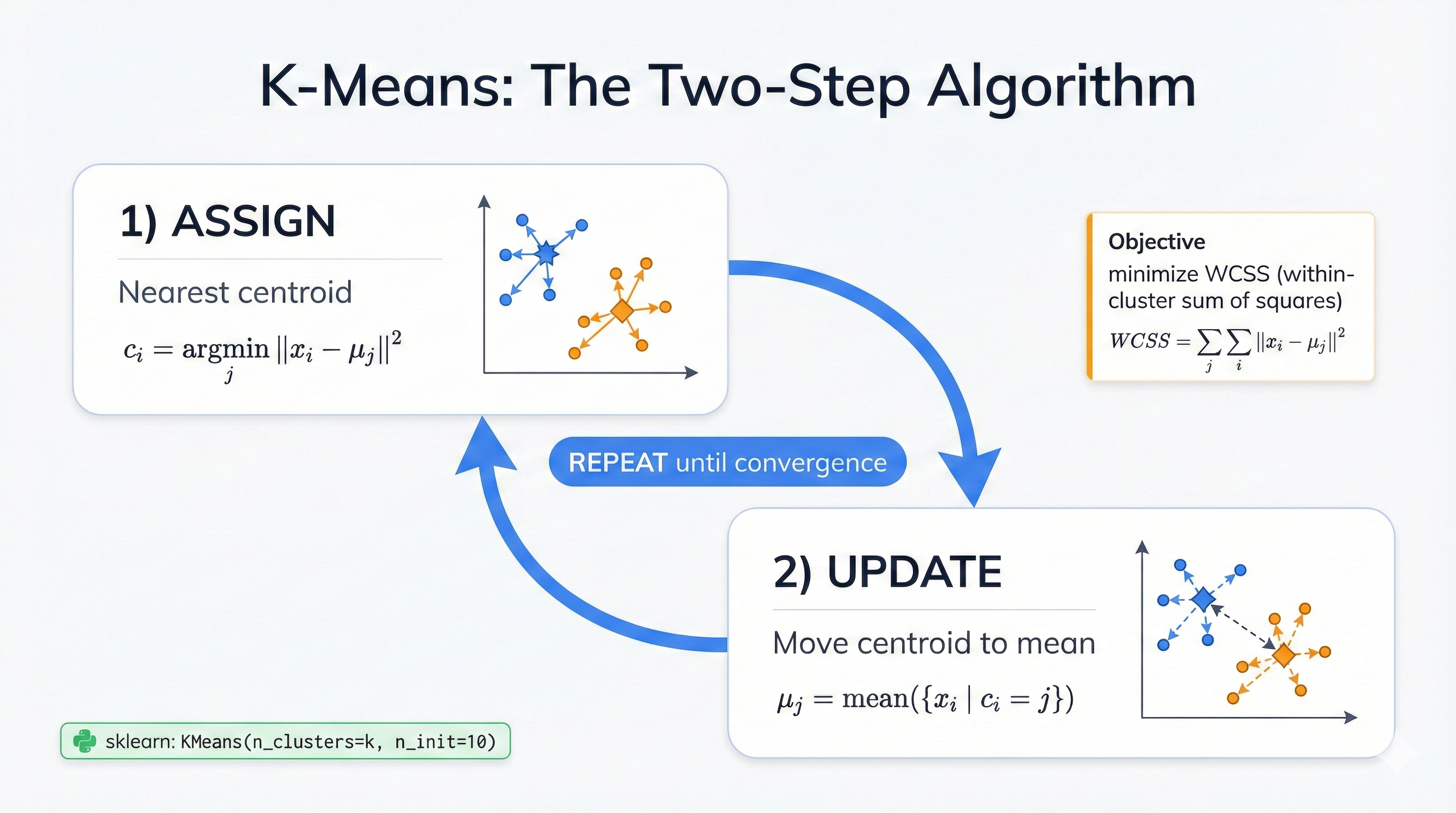
Two steps. That's it. First: assign each point to its nearest cluster center. Second: move each center to the average position of all its points. Keep going until nothing changes—when cluster centers stop their migration and points stop switching teams, you've reached convergence and discovered your data's natural groupings.
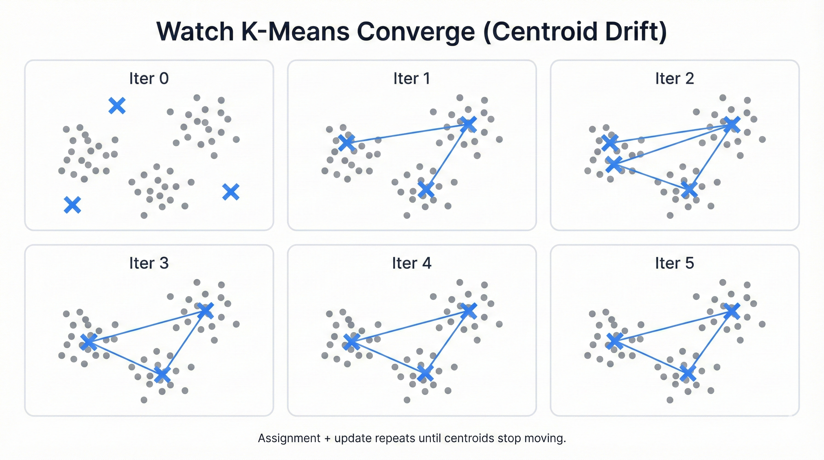
Watch K-Means Work: Step-by-Step Visualization
Want to see the magic? This code reveals everything. Watch cluster centers drift across the data landscape. See points jump between teams. Observe the algorithm's inexorable march toward optimal groupings, each iteration bringing greater clarity and tighter clusters.
import numpy as np
import matplotlib.pyplot as plt
from sklearn.cluster import KMeans
from sklearn.datasets import make_blobs

# Generate sample data with 3 natural clusters
np.random.seed(42)
X, y_true = make_blobs(n_samples=300, centers=3, cluster_std=1.2,
                      random_state=42)

print("K-Means Clustering Step-by-Step Demo")
print("=" * 40)
print(f"Dataset: {X.shape[0]} points, {X.shape[1]} dimensions")
print(f"Target: Find {len(np.unique(y_true))} clusters")
print()

# Initialize K-Means
kmeans = KMeans(n_clusters=3, init='random', n_init=1, max_iter=1, random_state=42)

# Store initial centroids by fitting once
kmeans.fit(X)
initial_centroids = kmeans.cluster_centers_.copy()

# Now demonstrate multiple iterations
fig, axes = plt.subplots(2, 3, figsize=(15, 10))
axes = axes.ravel()

# Show iterations
for iteration in range(6):
    # Fit with limited iterations
    kmeans = KMeans(n_clusters=3, init=initial_centroids, n_init=1,
                   max_iter=iteration+1, random_state=42)
    kmeans.fit(X)

    # Get cluster assignments and centroids
    labels = kmeans.labels_
    centroids = kmeans.cluster_centers_

    # Plot
    ax = axes[iteration]

    # Plot data points colored by cluster assignment
    colors = ['red', 'blue', 'green']
    for i in range(3):
        cluster_points = X[labels == i]
        ax.scatter(cluster_points[:, 0], cluster_points[:, 1],
                  c=colors[i], alpha=0.6, s=30)

    # Plot centroids
    ax.scatter(centroids[:, 0], centroids[:, 1], c='black',
              marker='x', s=200, linewidths=3, label='Centroids')

    # Calculate and display WCSS (Within-Cluster Sum of Squares)
    wcss = kmeans.inertia_
    ax.set_title(f'Iteration {iteration + 1}\nWCSS: {wcss:.1f}')
    ax.set_xlabel('Feature 1')
    ax.set_ylabel('Feature 2')
    ax.grid(True, alpha=0.3)

    if iteration == 0:
        ax.legend()

plt.tight_layout()
plt.show()

# Demonstrate the two-step process
print("\nTwo-Step K-Means Process:")
print("1. ASSIGNMENT STEP: Assign each point to nearest centroid")
print("2. UPDATE STEP: Move centroids to center of assigned points")
print("3. REPEAT until convergence (centroids stop moving)")

# Show final results
final_kmeans = KMeans(n_clusters=3, random_state=42)
final_kmeans.fit(X)

print(f"\nFinal Results:")
print(f"Converged in {final_kmeans.n_iter_} iterations")
print(f"Final WCSS: {final_kmeans.inertia_:.1f}")
print("\nFinal Centroids:")
for i, centroid in enumerate(final_kmeans.cluster_centers_):
    print(f"  Cluster {i}: ({centroid[0]:.2f}, {centroid[1]:.2f})")
Cluster centers migrate. Points switch allegiances. The algorithm iterates relentlessly until it achieves stability—when no point wants to jump to a different cluster and no center needs to move to better serve its members, the process ends and your clusters are born.
This dance comes from 1950s signal processing. The math proves that every iteration improves the solution. You can't get worse—only better or stuck at a local optimum, which is why running K-Means multiple times with different starting positions helps you avoid settling for mediocre groupings when spectacular ones might exist just around the corner.
Here's the two-step heartbeat:
Step 1 - Assignment: Every point joins its nearest center. Distance means Euclidean distance—straight-line measurement in your feature space. This creates invisible territories around each center, like medieval kingdoms where every citizen lives closest to their capital city and naturally belongs to that realm.
Step 2 - Update: Calculate new centers by averaging all points in each cluster. This pulls centers toward their members' center of mass. Clusters get tighter. Groups get more compact. The quality improves with every iteration, steadily marching toward an optimal arrangement that minimizes the total distance between points and their assigned cluster centers.
Stop when points stop switching. Stop when centers barely move. Stop when you hit 300 iterations. These convergence criteria ensure the algorithm finishes in reasonable time while still finding high-quality cluster arrangements that meaningfully organize your data.
Why K-Means Works the Way It Does
Bell Labs, 1957. Stuart Lloyd faced a problem. How do you convert continuous phone signals into discrete digital values without losing quality? The answer became K-Means—an algorithm that would eventually revolutionize machine learning, data mining, and computer vision decades after its humble birth in telecommunications research.
Lloyd needed representative points. A few digital values that could reconstruct analog signals with minimal error. K-Means found those points by clustering similar signal values together and using cluster centers as the reconstruction values—brilliant in its simplicity, powerful in its effectiveness, and perfectly suited for the emerging digital age.
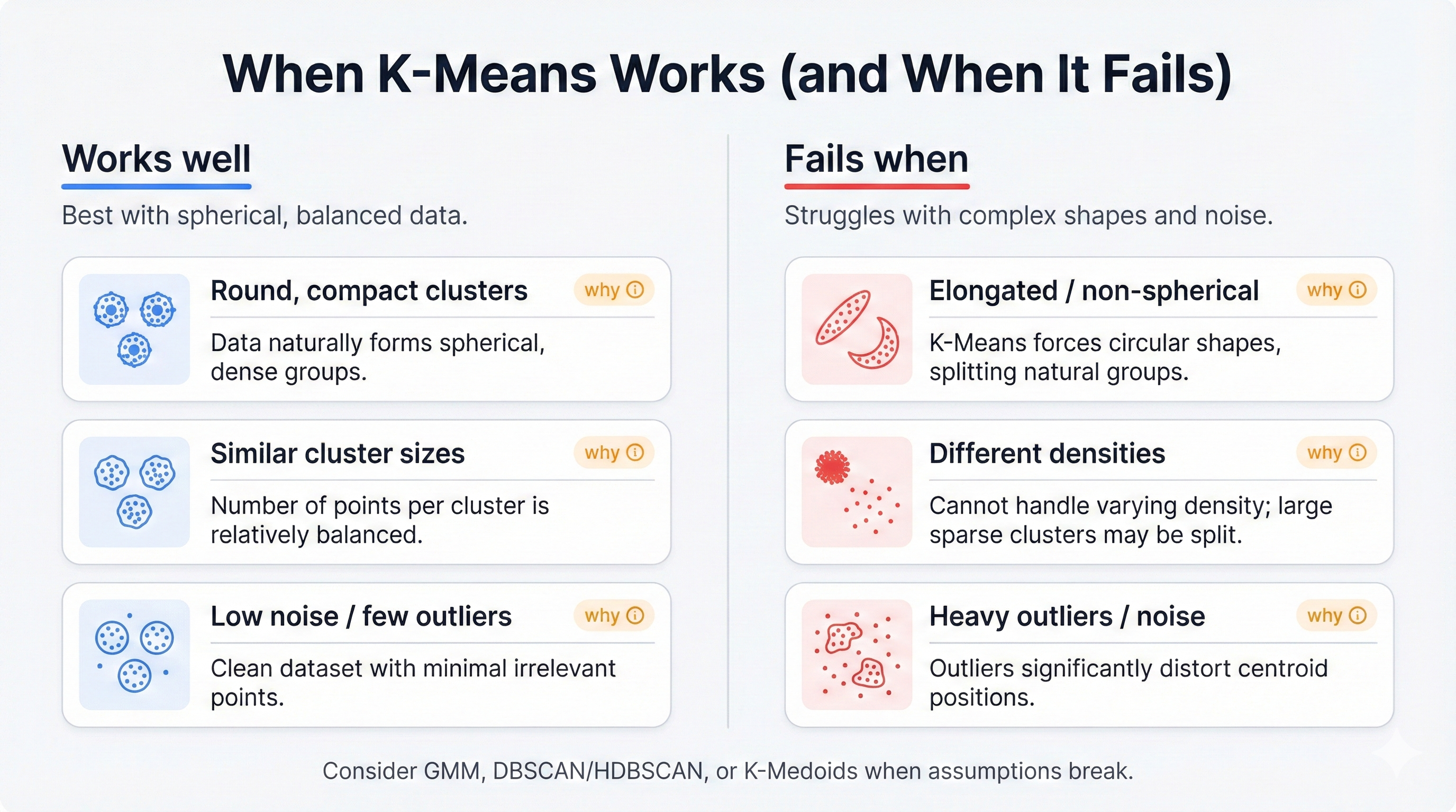
This origin explains everything. The algorithm minimizes reconstruction error, not natural groupings. Its preference for round, similarly-sized clusters comes from signal processing, not data science—which is why you need to understand these biases before applying K-Means to your business problems or risk discovering meaningless patterns that reflect the algorithm's assumptions rather than your data's true structure.
James MacQueen named it "k-means" in 1967, though Lloyd invented the core idea ten years earlier. Lloyd's original work? Buried in internal Bell Labs reports until 1982, when it finally reached public eyes and the world recognized the genius that had been hiding in plain sight for a quarter century.
K-Means in the Machine Learning Family Tree
Pure unsupervised learning. No labels guide it. No supervision constrains it. You dump raw data into K-Means and it discovers structure completely independently, finding patterns and groupings that exist naturally in your data without any prior knowledge of what those groupings should look like or what they might represent.
Two defining traits:
Hard Partitioning: Each point belongs to exactly one cluster. No fuzzy memberships. No probability distributions. You get clear, definitive assignments—point A belongs to cluster 1, point B belongs to cluster 2, with no ambiguity or shared membership between groups.
Fixed Cluster Count: You choose k upfront. K-Means then creates exactly that many groups, whether it makes sense or not. Pick k=5 and you'll get five clusters even if your data naturally contains three distinct groups or seven hidden segments—the algorithm forces your chosen number regardless of the underlying reality.
K-Means connects to sophisticated algorithms through shared math. It's a simplified Gaussian Mixture Model with harsh constraints: all clusters must be circular, identically sized, and equally probable. These assumptions make K-Means fast and simple but blind to complex real-world patterns that violate these strict requirements.
Relax the constraints? You unlock power. Allow elliptical clusters and you get Gaussian Mixture Models that handle elongated groupings. Use different distance metrics and you get K-Medoids that resist outliers. This makes K-Means your gateway drug to advanced clustering—learn it first, then graduate to more sophisticated techniques when its assumptions fail.
The Math Behind K-Means
K-Means pursues one goal. Minimize Within-Cluster Sum of Squares. WCSS measures cluster tightness—how close points huddle around their centers, with lower scores indicating more compact, homogeneous groups where members truly resemble each other and outliers are minimized.
What WCSS Actually Measures
Add up squared distances. From each point to its cluster center. Small WCSS means tight clusters. The algorithm relentlessly adjusts centers to drive this number down, iteration by iteration, until it reaches the lowest possible value given your chosen number of clusters and the algorithm's spherical cluster assumptions.
See WCSS Optimization in Action
import numpy as np
import matplotlib.pyplot as plt
from sklearn.cluster import KMeans
from sklearn.datasets import make_blobs

# Generate sample data
np.random.seed(42)
X, _ = make_blobs(n_samples=150, centers=3, cluster_std=1.0, random_state=42)

def calculate_wcss(X, centroids, labels):
    """Calculate Within-Cluster Sum of Squares manually"""
    wcss = 0
    for i in range(len(centroids)):
        cluster_points = X[labels == i]
        if len(cluster_points) > 0:
            distances_squared = np.sum((cluster_points - centroids[i])**2, axis=1)
            wcss += np.sum(distances_squared)
    return wcss

print("WCSS Minimization Demonstration")
print("=" * 35)

# Test different number of clusters
k_values = range(1, 8)
wcss_values = []

for k in k_values:
    kmeans = KMeans(n_clusters=k, random_state=42, n_init=10)
    kmeans.fit(X)

    # Built-in WCSS (inertia)
    wcss_sklearn = kmeans.inertia_

    # Manual calculation for verification
    wcss_manual = calculate_wcss(X, kmeans.cluster_centers_, kmeans.labels_)

    wcss_values.append(wcss_sklearn)

    print(f"k={k}: WCSS = {wcss_sklearn:.1f} (Manual: {wcss_manual:.1f})")

# Plot the elbow curve
fig, (ax1, ax2) = plt.subplots(1, 2, figsize=(14, 5))

# Elbow plot
ax1.plot(k_values, wcss_values, 'bo-', linewidth=2, markersize=8)
ax1.set_xlabel('Number of Clusters (k)')
ax1.set_ylabel('Within-Cluster Sum of Squares (WCSS)')
ax1.set_title('Elbow Method: WCSS vs k')
ax1.grid(True, alpha=0.3)

# Annotate the elbow point
elbow_point = 3  # Based on visual inspection
ax1.annotate(f'Elbow at k={elbow_point}',
            xy=(elbow_point, wcss_values[elbow_point-1]),
            xytext=(elbow_point+1, wcss_values[elbow_point-1]+500),
            arrowprops=dict(arrowstyle='->', color='red', lw=2),
            fontsize=12, color='red')

# Show optimal clustering
optimal_kmeans = KMeans(n_clusters=3, random_state=42)
optimal_kmeans.fit(X)
labels = optimal_kmeans.labels_
centroids = optimal_kmeans.cluster_centers_

colors = ['red', 'blue', 'green']
for i in range(3):
    cluster_points = X[labels == i]
    ax2.scatter(cluster_points[:, 0], cluster_points[:, 1],
               c=colors[i], alpha=0.6, s=50, label=f'Cluster {i}')

    # Draw lines from points to centroids to show distances
    for point in cluster_points[::10]:  # Every 10th point for clarity
        ax2.plot([point[0], centroids[i][0]], [point[1], centroids[i][1]],
                'gray', alpha=0.3, linewidth=0.5)

# Plot centroids
ax2.scatter(centroids[:, 0], centroids[:, 1], c='black', marker='x',
           s=300, linewidths=4, label='Centroids')
ax2.set_xlabel('Feature 1')
ax2.set_ylabel('Feature 2')
ax2.set_title(f'Optimal Clustering (k=3)\nWCSS = {optimal_kmeans.inertia_:.1f}')
ax2.legend()
ax2.grid(True, alpha=0.3)

plt.tight_layout()
plt.show()

print(f"\nKey Insight: K-Means minimizes the sum of squared distances")
print(f"from each point to its assigned centroid.")
print(f"\nMathematical Objective: J = Σᵢ Σₓ∈Sᵢ ||x - μᵢ||²")
print(f"Where μᵢ is the centroid of cluster Sᵢ")
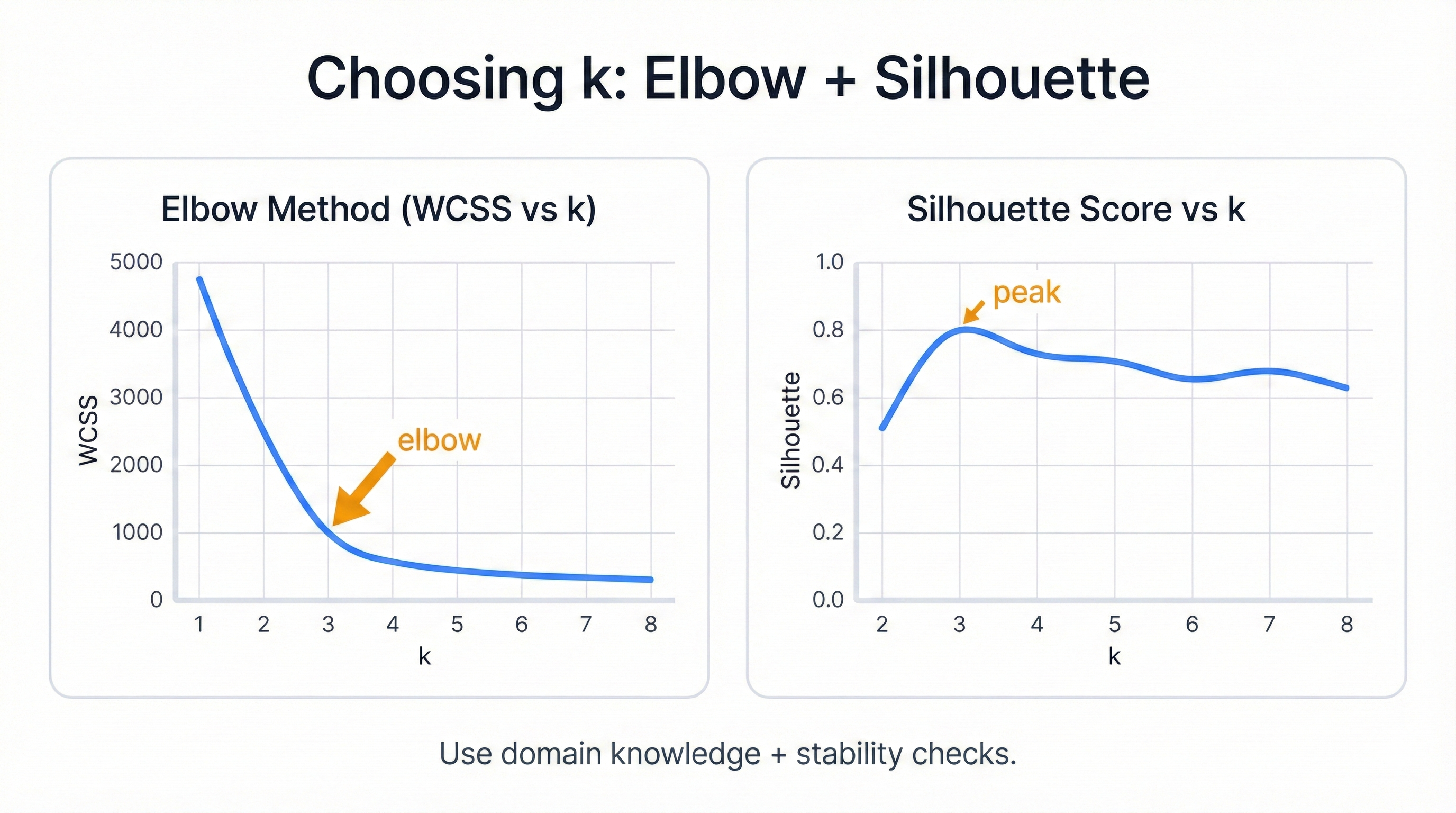
Watch WCSS plummet. The algorithm systematically reduces cluster scatter through optimal center placement. The elbow method emerges—a visual tool for choosing k by finding where WCSS reduction slows dramatically, indicating you've discovered the natural number of groups hiding in your data.
The math breaks down simply. You have n data points. You divide them into k groups. For each group, you calculate the center by averaging all member points. Then you measure scatter—the sum of squared distances from points to their centers, aggregated across all clusters into one powerful metric.
WCSS looks scary. It's not. For each cluster, measure distances from points to the center, square those distances to penalize outliers heavily, and add everything up. Repeat for all clusters. The result tells you how compact and homogeneous your groupings are, with lower values always indicating better cluster quality.
Mathematically: J = Σᵢ Σₓ∈Sᵢ ||x - μᵢ||²
μᵢ represents the cluster i centroid. Calculate it by averaging all points assigned to that cluster. This center minimizes squared distances to its members—a mathematical guarantee that comes from basic calculus and makes the mean the perfect choice for K-Means cluster centers.
Squared distances create round clusters. Outliers get punished exponentially. A point twice as far contributes four times the error, creating strong pressure for compact, spherical groupings where every member stays close to the center and deviations are minimized.
Here's the insight that blows minds: minimize within-cluster scatter and you automatically maximize between-cluster separation. Total variation stays constant. Tighter clusters mean more distinct groups. It's a beautiful mathematical symmetry that makes K-Means simultaneously optimize for both cluster cohesion and separation in a single unified objective function.
Squared Euclidean distance pairs perfectly with the mean. The mean minimizes squared distances—a proven mathematical fact. This creates a feedback loop where the distance metric and centroid calculation method reinforce each other, guaranteeing convergence to at least a local optimum every single time you run the algorithm.
Change the distance metric? You need a different algorithm. Manhattan distance requires the median as center, giving you K-Medoids. Maximum distance needs a different optimization entirely. The choice of metric fundamentally determines what "center" means and how clusters form.
Getting Your Data Ready for K-Means
K-Means is picky. Feed it bad data? Get worthless results. The algorithm assumes your data is clean, scaled, and numerical—violate these assumptions and you'll waste hours chasing phantom patterns that exist only because you skipped preprocessing.
What Kind of Data Works
Numbers Only: K-Means demands continuous numerical features. No categories. No text. No missing values. Got mixed types? Try K-Prototypes—it handles both numbers and categories, expanding K-Means' usefulness to datasets that combine numerical measurements with categorical attributes like product types or customer segments.
Feature Scaling: The Most Important Step
import numpy as np
import matplotlib.pyplot as plt
from sklearn.cluster import KMeans
from sklearn.preprocessing import StandardScaler, MinMaxScaler
from sklearn.datasets import make_blobs

# Create synthetic dataset with features on different scales
np.random.seed(42)
n_samples = 200

# Generate base data
X_base, y_true = make_blobs(n_samples=n_samples, centers=3,
                           cluster_std=1.0, random_state=42)

# Create features with dramatically different scales
# Feature 1: Age (20-70)
age = 20 + (X_base[:, 0] - X_base[:, 0].min()) / (X_base[:, 0].max() - X_base[:, 0].min()) * 50

# Feature 2: Income (20,000-200,000) - much larger scale
income_base = (X_base[:, 1] - X_base[:, 1].min()) / (X_base[:, 1].max() - X_base[:, 1].min())
income = 20000 + income_base * 180000

# Combine into unscaled dataset
X_unscaled = np.column_stack([age, income])

print("Feature Scaling Impact on K-Means Clustering")
print("=" * 45)
print(f"Age range: {age.min():.0f} - {age.max():.0f}")
print(f"Income range: ${income.min():.0f} - ${income.max():.0f}")
print(f"Income scale is ~{income.max()/age.max():.0f}x larger than age!")
print()

# Apply different scaling methods
scaler_standard = StandardScaler()
scaler_minmax = MinMaxScaler()

X_standardized = scaler_standard.fit_transform(X_unscaled)
X_minmax = scaler_minmax.fit_transform(X_unscaled)

# Cluster with each version
kmeans_unscaled = KMeans(n_clusters=3, random_state=42, n_init=10)
kmeans_standard = KMeans(n_clusters=3, random_state=42, n_init=10)
kmeans_minmax = KMeans(n_clusters=3, random_state=42, n_init=10)

labels_unscaled = kmeans_unscaled.fit_predict(X_unscaled)
labels_standard = kmeans_standard.fit_predict(X_standardized)
labels_minmax = kmeans_minmax.fit_predict(X_minmax)

# Compare clustering quality
from sklearn.metrics import silhouette_score, calinski_harabasz_score

print("Clustering Quality Metrics:")
print("-" * 30)

metrics = [
    ("Unscaled", X_unscaled, labels_unscaled),
    ("Standardized", X_standardized, labels_standard),
    ("Min-Max Scaled", X_minmax, labels_minmax)
]

for name, X_data, labels in metrics:
    sil_score = silhouette_score(X_data, labels)
    ch_score = calinski_harabasz_score(X_data, labels)
    wcss = KMeans(n_clusters=3, random_state=42).fit(X_data).inertia_

    print(f"{name:15} | Silhouette: {sil_score:.3f} | CH Index: {ch_score:.1f} | WCSS: {wcss:.1f}")

print("\nKey Takeaway: Without scaling, income dominates clustering entirely!")
print("Proper scaling ensures all features contribute meaningfully.")
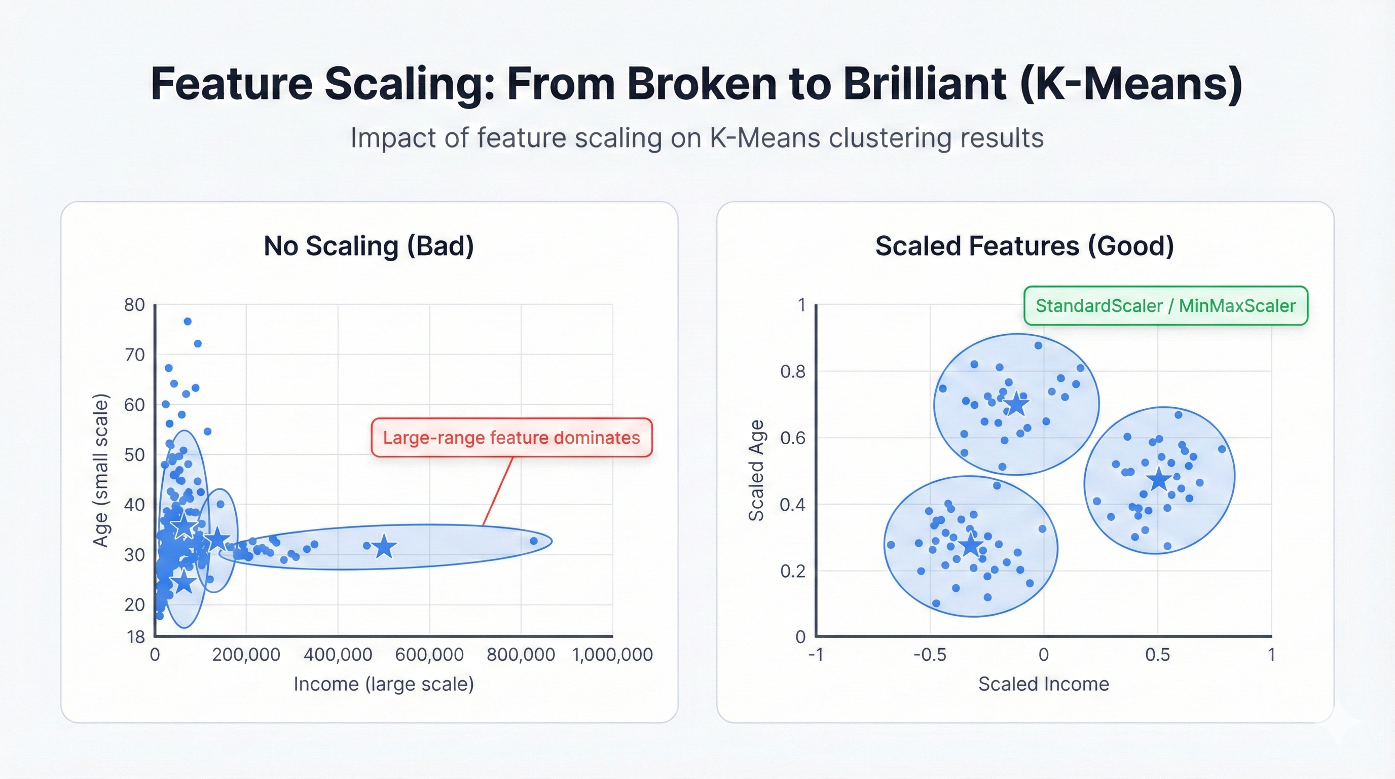
Feature scaling transforms K-Means from broken to brilliant. Without it, high-magnitude features dominate completely, rendering small-scale features invisible to the algorithm. With it, every feature contributes equally to the clustering decision, revealing patterns that would otherwise stay hidden beneath scale imbalances.
Feature Scaling is Mandatory: K-Means uses Euclidean distance. Features with large ranges dominate ruthlessly. Income ranging 20,000-200,000 versus age ranging 20-70? Income controls everything. Age becomes irrelevant. Your clusters reflect only income while completely ignoring age—a disaster if age matters for your business problem.
Two scaling approaches dominate:
- Standardization (Z-score): Centers features at zero. Sets standard deviation to one. Handles outliers gracefully.
- Min-Max Scaling: Rescales features to 0-1 range. Preserves original distribution shape. Sensitive to outliers.
Handle Missing Values: K-Means breaks with missing data. It can't calculate distances to incomplete points. Fix this first through imputation, deletion, or switching to algorithms that handle missing values natively—there's no way around this hard requirement.
Real-World Applications: Where K-Means Shines
K-Means solves real problems. Not toy examples. Not academic exercises. Actual business challenges that generate revenue, reduce costs, and create competitive advantages across every industry from retail to healthcare to finance.
E-Commerce Customer Segmentation Example
import numpy as np
import pandas as pd
from sklearn.cluster import KMeans
from sklearn.preprocessing import StandardScaler
import matplotlib.pyplot as plt

# Simulate customer data with RFM analysis
np.random.seed(42)
n_customers = 1000

# Generate customer features: Recency, Frequency, Monetary
recency = np.random.exponential(30, n_customers)  # Days since last purchase
frequency = np.random.poisson(5, n_customers)    # Number of purchases
monetary = np.random.gamma(2, 100, n_customers)  # Total spending

# Create customer dataframe
customers = pd.DataFrame({
    'CustomerID': range(1, n_customers + 1),
    'Recency': recency,
    'Frequency': frequency,
    'Monetary': monetary
})

# Standardize features for clustering
scaler = StandardScaler()
X_scaled = scaler.fit_transform(customers[['Recency', 'Frequency', 'Monetary']])

# Apply K-Means clustering
kmeans = KMeans(n_clusters=4, random_state=42, n_init=10)
customers['Segment'] = kmeans.fit_predict(X_scaled)

# Analyze segment characteristics
segment_analysis = customers.groupby('Segment').agg({
    'Recency': ['mean', 'std'],
    'Frequency': ['mean', 'std'],
    'Monetary': ['mean', 'std']
}).round(2)

# Business interpretation of segments
segment_labels = {
    0: "Champions (High Value, Active)",
    1: "Loyal Customers (Regular, Moderate Value)",
    2: "Potential Loyalists (Recent, Low Frequency)",
    3: "At Risk (High Recency, Low Activity)"
}

print("Customer Segmentation Results:")
for segment in range(4):
    print(f"\n{segment_labels[segment]}:")
    print(f"  Avg Recency: {segment_analysis.loc[segment, ('Recency', 'mean')]:.1f} days")
    print(f"  Avg Frequency: {segment_analysis.loc[segment, ('Frequency', 'mean')]:.1f} purchases")
    print(f"  Avg Monetary: ${segment_analysis.loc[segment, ('Monetary', 'mean')]:.0f}")
    print(f"  Size: {(customers['Segment'] == segment).sum()} customers")
Raw data becomes business intelligence. K-Means transforms customer transaction history into actionable segments that drive marketing strategy, with each group receiving tailored treatment designed for their specific behavior pattern—Champions get VIP perks, Loyal Customers earn loyalty rewards, Potential Loyalists see engagement campaigns, and At-Risk customers receive win-back offers that could prevent churn and recover revenue. Standardization proves crucial because days, dollars, and purchase counts exist on wildly different scales that would otherwise make clustering impossible.
Conclusion: K-Means in Practice
Best Practice: Following these recommended practices will help you achieve optimal results and avoid common pitfalls.
Sixty years later, K-Means survives. It thrives. Born in 1950s signal processing labs, it has become the default choice for unsupervised learning—simple enough for beginners, powerful enough for production systems, and fast enough to handle massive datasets that would choke more sophisticated algorithms.
Why K-Means Endures
Simplicity wins. Assign points to nearest centers, move centers to point averages, repeat until stable—this intuitive process scales linearly with data size and produces results anyone can interpret, making it the perfect tool for everything from customer segmentation to image compression to document clustering to anomaly detection to recommendation systems.
Understanding the Trade-offs
K-Means makes assumptions. Harsh ones. Clusters should be round, similarly-sized, and well-separated. Violate these rules? Get garbage results. The algorithm demands you choose k upfront and can get trapped in poor local minima that miss the global optimum—these aren't bugs but design decisions that enable the algorithm's speed and simplicity.
Speed costs flexibility. Simplicity costs sophistication. These trade-offs aren't flaws but conscious design choices. Modern improvements like K-Means++ initialization and variants like K-Medoids address many limitations while keeping the core advantages that make K-Means so valuable for real-world applications.
The Future Looks Bright
Research continues. Automatic k selection removes the guessing game. Deep learning integration adds representational power. LLM-powered semantic clustering enables context-aware groupings that understand meaning, not just mathematical distance. Cloud platforms democratize sophisticated clustering through AutoML features that make expert-level results accessible to everyone regardless of their data science background.
Success Recipe
Master K-Means through five steps:
- Understand your data - visualize first, check assumptions, spot outliers
- Preprocess carefully - scale features religiously, handle missing values properly
- Choose k wisely - use elbow method, silhouette analysis, domain knowledge
- Use proven settings - K-Means++ initialization, multiple runs, reasonable iteration limits
- Interpret results - profile centroids thoroughly, validate with domain experts
Apply K-Means within its strengths and it becomes indispensable for discovering hidden patterns, generating business insights, and solving real problems that directly impact your bottom line through better customer understanding, improved operational efficiency, and data-driven decision making that transforms raw information into competitive advantage.