1. An Introduction to Hierarchical Cluster Analysis
Think of trees. Hierarchical clustering builds them from your data. No guessing required—you won't spend hours wondering how many clusters exist, because the algorithm reveals natural structure at every single level of detail, from the finest granular distinctions to the broadest categorical groupings.
Key Concept: Understanding this foundational concept is essential for mastering the techniques discussed in this article.
The core principle works elegantly: objects sitting close together share more similarities than distant ones. Simple, right? This fundamental relationship creates a tree-like hierarchy that shows exactly how clusters merge or split at different levels, revealing patterns you'd miss with other techniques.
1.1 The Core Principle: Building Nested Cluster Structures
Here's the magic. Hierarchical clustering delivers every possible clustering solution in one tree structure. We call it a dendrogram.
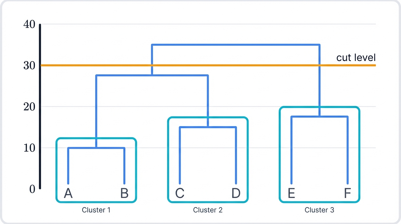
A dendrogram—Greek for "tree drawing"—displays your data as a tree where individual data points form leaves at the bottom, and moving up the tree, clusters progressively merge together in a cascade of increasingly abstract groupings. The height where clusters merge reveals their similarity: shorter merges connect more similar clusters, taller merges join less similar ones, and the difference between these heights tells you exactly how much similarity you're sacrificing as you move up the hierarchy.
Here's the key advantage. You examine the dendrogram first, then decide where to cut it. Make a horizontal "cut" at any level that makes sense—wherever you see the most dramatic separation, wherever your domain knowledge suggests a natural boundary, wherever the story in your data becomes clearest. Count the vertical lines you cross, and that equals your cluster count. This flexibility makes hierarchical clustering ideal for exploratory analysis when you're genuinely unsure about your data's underlying structure.
Working Example: Hierarchical Clustering Step-by-Step
Watch the complete process unfold. This example walks through hierarchical clustering from start to finish—calculating distances, building the tree, assigning final clusters.
import numpy as np
import matplotlib.pyplot as plt
from scipy.cluster.hierarchy import dendrogram, linkage, fcluster
from scipy.spatial.distance import pdist, squareform
from sklearn.datasets import make_blobs

# Generate sample data for demonstration
np.random.seed(42)
X, _ = make_blobs(n_samples=8, centers=3, cluster_std=1.0, random_state=42)

print("Hierarchical Clustering Step-by-Step Demonstration")
print("=" * 55)

# Step 1: Compute pairwise distance matrix
distances = pdist(X, metric='euclidean')
distance_matrix = squareform(distances)

print("Step 1: Pairwise Distance Matrix")
print("Points shape:", X.shape)
print("Distance matrix shape:", distance_matrix.shape)
print("Sample distances between first 3 points:")
for i in range(3):
    for j in range(3):
        if i != j:
            print(f"  Point {i} to Point {j}: {distance_matrix[i,j]:.3f}")

# Step 2: Perform hierarchical clustering with different linkage methods
linkage_methods = ['single', 'complete', 'average', 'ward']

for method in linkage_methods:
    print(f"\nStep 2: {method.capitalize()} Linkage Clustering")
    print("-" * 40)

    # Compute linkage matrix
    Z = linkage(X, method=method)

    print("Merge history (linkage matrix):")
    print("Format: [cluster1, cluster2, distance, size]")
    for i, merge in enumerate(Z):
        cluster1, cluster2, distance, size = merge
        print(f"  Merge {i+1}: Clusters {int(cluster1):2d} & {int(cluster2):2d} "
              f"→ distance {distance:.3f}, size {int(size)}")

    # Step 3: Cut dendrogram at different levels
    print(f"\nStep 3: Cutting dendrogram at different heights")
    cut_heights = [1.0, 2.0, 3.0]

    for height in cut_heights:
        clusters = fcluster(Z, height, criterion='distance')
        n_clusters = len(np.unique(clusters))
        print(f"  Cut at height {height:.1f}: {n_clusters} clusters")
        print(f"  Cluster assignments: {clusters}")

# Step 4: Compare linkage methods on their cluster formation
print(f"\nStep 4: Linkage Method Comparison")
print("-" * 35)

# Create a simple 2D example to visualize differences
simple_data = np.array([[0, 0], [1, 0], [0, 1], [5, 5], [6, 5], [5, 6]])

for method in ['single', 'complete', 'ward']:
    Z = linkage(simple_data, method=method)
    clusters_2 = fcluster(Z, 2, criterion='maxclust')
    clusters_3 = fcluster(Z, 3, criterion='maxclust')

    print(f"{method.capitalize()} linkage:")
    print(f"  2 clusters: {clusters_2}")
    print(f"  3 clusters: {clusters_3}")

# Step 5: Demonstrate the chaining effect in single linkage
print(f"\nStep 5: Chaining Effect Demonstration")
print("-" * 37)

# Create data with a "bridge" between clusters
cluster1 = np.array([[0, 0], [1, 0], [0, 1]])
bridge = np.array([[2.5, 0.5]])  # Bridge point
cluster2 = np.array([[5, 0], [6, 0], [5, 1]])
chaining_data = np.vstack([cluster1, bridge, cluster2])

for method in ['single', 'complete']:
    Z = linkage(chaining_data, method=method)
    clusters = fcluster(Z, 2, criterion='maxclust')
    print(f"{method.capitalize()} linkage with bridge point:")
    print(f"  Data points: {len(chaining_data)} total")
    print(f"  2-cluster solution: {clusters}")
    print(f"  Bridge effect: {'Present' if len(np.unique(clusters)) < 2 else 'Avoided'}")
This step-by-step example shows how hierarchical clustering constructs its dendrogram through repeated merges. Single linkage suffers from the notorious "chaining effect"—outlier points create bridges between distinct clusters, joining groups that should remain separate. Ward's method builds compact, balanced clusters by minimizing variance at each merge. The linkage matrix tracks the complete merge history, so you can cut at any level you want and extract whatever cluster granularity makes sense for your analysis.
1.2 Two Directions: Agglomerative vs. Divisive Approaches
Hierarchical clustering operates in two directions. Bottom-up or top-down. Agglomerative or divisive.
1.2.1 Agglomerative Clustering (Bottom-Up)
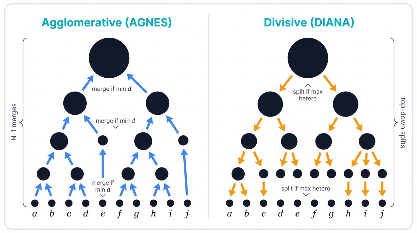
Agglomerative clustering dominates the field. It goes by the acronym AGNES—AGglomerative NESting. You start with every data point as its own cluster, then repeatedly merge the two most similar clusters until everything belongs to one giant cluster, building your tree from the leaves upward in a series of progressive consolidations.
The algorithm performs N-1 merges for N data points. Each merge decision creates one level of your dendrogram tree, and the beauty lies in this simplicity—no complex optimization, just greedy local decisions that build a global structure.
1.2.2 Divisive Clustering (Top-Down)
Divisive clustering works backwards. DIANA—DIvisive ANAlysis. You start with all data in one massive cluster, then repeatedly split the most heterogeneous cluster into smaller, more cohesive pieces, continuing this top-down fracturing until every point sits in its own isolated cluster.
Divisive clustering proves computationally harder. Less popular too. The reason? Exponentially many ways exist to split any cluster into two parts—the combinatorial explosion is real, and you need clever heuristics like using K-Means for the splits or finding the two most dissimilar points as seeds to make the problem tractable.
Despite this complexity, divisive clustering identifies large, distinct clusters early since it considers the global data distribution from the start, rather than building up from local similarities like its agglomerative cousin.
1.3 Historical Foundations: From Social Science to Computing
Clustering predates computers by decades. It emerged in early 20th-century social sciences. Driver and Kroeber pioneered quantitative methods for cultural typologies in 1932. Psychology advanced these ideas through Robert Tryon's cluster analysis in 1939 and Raymond Cattell's personality trait classification in 1943—all done by hand, with painstaking calculations that make modern computational approaches seem miraculous.
Computational formalization occurred in the 1960s during rapid statistical computing development, when researchers finally had machines powerful enough to handle the calculations. Joe H. Ward Jr. created the landmark Ward's method in 1963—it minimizes within-cluster sum of squares increase at each merge, providing a principled objective function that still dominates practice today. Macnaughton-Smith established divisive clustering principles in 1964, later refined by Kaufman and Rousseeuw's DIANA algorithm in 1990.
Early algorithm design reflected computational constraints. The iterative, greedy nature exists because merges and splits remain final—they can't be undone, avoiding the combinatorial explosion that would have overwhelmed 1960s-era computers. This historical context explains why classical methods have both their enduring strengths and inherent limitations.
1.4 Hierarchical Clustering in the Unsupervised Learning Paradigm
Hierarchical clustering exemplifies unsupervised learning. You get no labels. No target variables. Just raw, unlabeled data. Your sole objective: discover hidden structures and natural groupings based on intrinsic data properties alone, finding patterns the data wants to reveal rather than patterns you've told it to find. This differs fundamentally from supervised learning where classification and regression map inputs to known outputs, and from reinforcement learning where agents maximize cumulative rewards through trial and error.
Dendrograms make powerful exploratory tools, but they can deceive you visually—the algorithm creates hierarchical structure even with random data that lacks any inherent clusters whatsoever. A dendrogram's existence doesn't prove meaningful groups exist in your data. Always pair visual interpretation with quantitative validation metrics to separate real structure from algorithmic artifacts. The greedy, path-dependent nature means early locally optimal merges can create globally suboptimal hierarchies, and this fundamental limitation drove development of advanced, more robust variants that we'll explore throughout this guide.
2. Algorithmic and Mathematical Architecture
Hierarchical clustering mechanics rest on two pillars: distance measurement and inter-cluster proximity rules. Your specific choices determine algorithm behavior and final hierarchy structure in ways that dramatically reshape your results.
2.1 The Dissimilarity Matrix Foundation
Hierarchical clustering doesn't use raw data directly. It requires a pairwise dissimilarity matrix. For N data points, you get an N×N symmetric matrix where entry (i,j) represents dissimilarity between points i and j—a complete map of every relationship in your dataset.
Pre-computed distance matrices provide tremendous flexibility. The algorithm decouples from data representation—it works with any domain where meaningful distance or dissimilarity measures exist, liberating you from the tyranny of vector spaces. This includes not just traditional vector space points, but complex data types: strings compared by edit distance, DNA sequences aligned by biological similarity, graphs measured by structural equivalence.
2.2 Distance Metrics: Quantifying Separation
Your chosen distance metric populates the dissimilarity matrix. This critical decision directly influences what counts as "similar" and shapes the entire clustering outcome—change the metric, change the clusters.
Euclidean Distance (L₂ norm) represents the most common metric. Straight-line distance between points in multi-dimensional space. This metric works perfectly for continuous, dense data with compact, globular clusters where traditional geometric distance relationships apply, giving you intuitive results that match spatial reasoning.
Manhattan Distance (L₁ norm) calculates city block distance by summing absolute coordinate differences. More robust than Euclidean distance in high dimensions and when dealing with outliers that might skew traditional distance calculations, it excels when your features represent independent quantities that shouldn't interact geometrically.
Cosine Similarity and Distance measures the cosine of the angle between non-zero vectors, ignoring magnitude while focusing purely on orientation—direction matters, size doesn't. This metric excels for high-dimensional data like text documents where word proportions matter infinitely more than document length, and you can convert similarity to distance using the simple formula: distance = 1 - similarity.
Working Example: Distance Metrics Comparison
import numpy as np
from scipy.spatial.distance import pdist, squareform
from scipy.cluster.hierarchy import linkage, dendrogram, fcluster
import matplotlib.pyplot as plt

# Create test data with different characteristics
np.random.seed(42)

# Dataset 1: Compact clusters (good for Euclidean)
compact_data = np.array([
    [1, 1], [1.2, 1.1], [0.9, 1.1],    # Cluster 1
    [5, 5], [5.1, 5.2], [4.9, 4.8],    # Cluster 2
    [1, 5], [1.1, 5.1], [0.9, 4.9]     # Cluster 3
])

# Dataset 2: Elongated clusters (good for Manhattan)
elongated_data = np.array([
    [0, 0], [1, 0], [2, 0], [3, 0],    # Horizontal cluster
    [0, 3], [0, 4], [0, 5], [0, 6],    # Vertical cluster
    [6, 6], [7, 6], [8, 6], [9, 6]     # Another horizontal cluster
])

# Dataset 3: High-dimensional sparse data (good for Cosine)
# Simulate document vectors with few non-zero entries
doc_vectors = np.array([
    [1, 0, 1, 0, 1, 0, 0, 0, 0, 0],    # Doc type A
    [1, 0, 0, 1, 1, 0, 0, 0, 0, 0],    # Doc type A
    [0, 1, 0, 0, 0, 1, 1, 0, 0, 0],    # Doc type B
    [0, 1, 0, 0, 0, 0, 1, 1, 0, 0],    # Doc type B
    [0, 0, 0, 0, 0, 0, 0, 0, 1, 1],    # Doc type C
    [0, 0, 0, 0, 0, 0, 0, 0, 1, 0]     # Doc type C
])

datasets = [
    ("Compact Clusters", compact_data),
    ("Elongated Clusters", elongated_data),
    ("Document Vectors", doc_vectors)
]

distance_metrics = ['euclidean', 'manhattan', 'cosine']

print("Distance Metrics Comparison on Different Data Types")
print("=" * 55)

for dataset_name, data in datasets:
    print(f"\nDataset: {dataset_name}")
    print("-" * (len(dataset_name) + 9))

    for metric in distance_metrics:
        print(f"\n{metric.capitalize()} Distance:")

        # Compute pairwise distances
        try:
            distances = pdist(data, metric=metric)
            distance_matrix = squareform(distances)

            # Perform hierarchical clustering
            Z = linkage(data, metric=metric, method='average')

            # Get 3 clusters
            clusters = fcluster(Z, 3, criterion='maxclust')
            unique_clusters = len(np.unique(clusters))

            print(f"  Cluster assignments (3 desired): {clusters}")
            print(f"  Actual clusters formed: {unique_clusters}")

            # Calculate average within-cluster vs between-cluster distances
            within_distances = []
            between_distances = []

            for i in range(len(data)):
                for j in range(i+1, len(data)):
                    if clusters[i] == clusters[j]:
                        within_distances.append(distance_matrix[i, j])
                    else:
                        between_distances.append(distance_matrix[i, j])

            if within_distances:
                avg_within = np.mean(within_distances)
                print(f"  Avg within-cluster distance: {avg_within:.3f}")

            if between_distances:
                avg_between = np.mean(between_distances)
                print(f"  Avg between-cluster distance: {avg_between:.3f}")

            if within_distances and between_distances:
                separation_ratio = avg_between / avg_within
                print(f"  Separation ratio: {separation_ratio:.2f}")

        except Exception as e:
            print(f"  Error with {metric}: {str(e)}")

# Demonstrate the impact of different distance metrics on clustering
print(f"\nKey Insights:")
print("- Euclidean works best for compact, spherical clusters")
print("- Manhattan is robust to outliers and works well with elongated clusters")
print("- Cosine focuses on direction, ideal for sparse high-dimensional data")
print("- Distance metric choice significantly affects clustering outcomes")
2.3 Linkage Criteria: Defining Inter-Cluster Distance
Once you have distances between individual points, you need rules for measuring distances between clusters containing multiple points. This is where linkage criteria become crucial—they define the very meaning of cluster proximity.
2.3.1 Single Linkage (Nearest Neighbor)
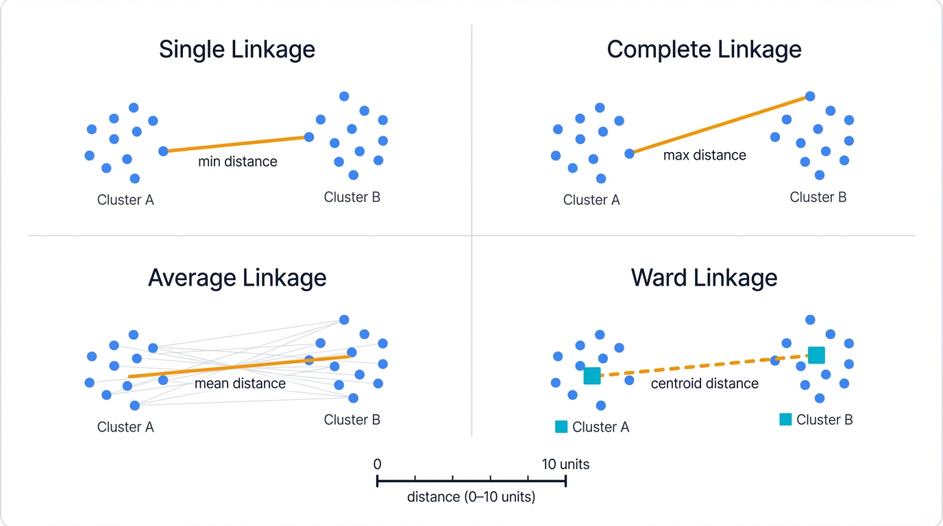
Single linkage defines inter-cluster distance as the minimum distance between any two points from different clusters. Mathematically:
$$d_{single}(C_i, C_j) = \min_{x \in C_i, y \in C_j} d(x, y)$$
This "nearest neighbor" approach creates elongated, chain-like clusters that can snake through your data space. It excels at detecting non-convex cluster shapes and connecting components through narrow bridges. However, single linkage suffers from the notorious "chaining effect"—a few outlier points can force separate clusters to merge prematurely, creating spurious connections that distort the true structure.
2.3.2 Complete Linkage (Furthest Neighbor)
Complete linkage uses the maximum distance between points from different clusters:
$$d_{complete}(C_i, C_j) = \max_{x \in C_i, y \in C_j} d(x, y)$$
This "furthest neighbor" criterion produces compact, roughly spherical clusters with similar diameters—think tight balls of data. It resists the chaining effect beautifully but struggles with elongated natural clusters and can be overly sensitive to outliers that inflate the maximum distance.
2.3.3 Average Linkage (UPGMA)
Average linkage computes the mean distance between all pairs of points from different clusters:
$$d_{average}(C_i, C_j) = \frac{1}{|C_i| \cdot |C_j|} \sum_{x \in C_i} \sum_{y \in C_j} d(x, y)$$
This balanced approach—UPGMA stands for Unweighted Pair Group Method with Arithmetic Mean—considers all inter-cluster relationships, reducing sensitivity to outliers while maintaining reasonable cluster shapes. It represents a sensible middle ground between single and complete linkage extremes, often performing well when you're unsure which extreme to choose.
2.3.4 Ward's Method (Minimum Variance)
Ward's method minimizes the increase in within-cluster sum of squared errors when merging clusters:
$$d_{ward}(C_i, C_j) = \sqrt{\frac{2|C_i||C_j|}{|C_i| + |C_j|}} \cdot ||μ_i - μ_j||_2$$
where $μ_i$ and $μ_j$ are cluster centroids. This variance-minimizing approach produces compact, well-balanced clusters with similar sizes—it's the statistician's favorite because it has a clear objective function. Ward's method works exclusively with Euclidean distances and tends to create spherical clusters, making it ideal when your data naturally forms round, evenly-sized groups.
Working Example: Linkage Criteria Comparison
import numpy as np
import matplotlib.pyplot as plt
from scipy.cluster.hierarchy import linkage, dendrogram, fcluster
from sklearn.datasets import make_blobs, make_moons
from sklearn.preprocessing import StandardScaler

# Create datasets with different characteristics
np.random.seed(42)

# Dataset 1: Well-separated circular clusters
circular_data, _ = make_blobs(n_samples=150, centers=3, cluster_std=1.5,
                              center_box=(-10.0, 10.0), random_state=42)

# Dataset 2: Non-convex moon shapes
moon_data, _ = make_moons(n_samples=150, noise=0.1, random_state=42)
moon_data = StandardScaler().fit_transform(moon_data)

# Dataset 3: Elongated clusters with different densities
elongated_cluster1 = np.random.multivariate_normal([0, 0], [[4, 0], [0, 1]], 50)
elongated_cluster2 = np.random.multivariate_normal([8, 8], [[1, 0], [0, 4]], 50)
elongated_cluster3 = np.random.multivariate_normal([0, 8], [[2, 1], [1, 2]], 50)
elongated_data = np.vstack([elongated_cluster1, elongated_cluster2, elongated_cluster3])

datasets = [
    ("Circular Clusters", circular_data, 3),
    ("Moon Shapes", moon_data, 2),
    ("Elongated Clusters", elongated_data, 3)
]

linkage_methods = ['single', 'complete', 'average', 'ward']

print("Linkage Criteria Comparison Across Different Data Types")
print("=" * 58)

for dataset_name, data, true_k in datasets:
    print(f"\nDataset: {dataset_name} (Expected {true_k} clusters)")
    print("-" * (len(dataset_name) + len(f" (Expected {true_k} clusters)") + 9))

    for method in linkage_methods:
        print(f"\n{method.capitalize()} Linkage:")

        try:
            # Perform hierarchical clustering
            Z = linkage(data, method=method)

            # Get clusters for the expected number
            clusters = fcluster(Z, true_k, criterion='maxclust')

            print(f"  Cluster sizes: {np.bincount(clusters)[1:]}")  # Skip 0 index

            # Calculate intra-cluster and inter-cluster statistics
            cluster_centers = []
            intra_cluster_distances = []

            for cluster_id in range(1, true_k + 1):
                cluster_points = data[clusters == cluster_id]
                if len(cluster_points) > 1:
                    center = np.mean(cluster_points, axis=0)
                    cluster_centers.append(center)

                    # Calculate average intra-cluster distance
                    distances = []
                    for i in range(len(cluster_points)):
                        for j in range(i+1, len(cluster_points)):
                            distances.append(np.linalg.norm(
                                cluster_points[i] - cluster_points[j]))

                    if distances:
                        intra_cluster_distances.append(np.mean(distances))

            if intra_cluster_distances:
                avg_intra = np.mean(intra_cluster_distances)
                print(f"  Average intra-cluster distance: {avg_intra:.3f}")

            # Calculate inter-cluster distances
            if len(cluster_centers) > 1:
                inter_distances = []
                for i in range(len(cluster_centers)):
                    for j in range(i+1, len(cluster_centers)):
                        inter_distances.append(np.linalg.norm(
                            cluster_centers[i] - cluster_centers[j]))

                avg_inter = np.mean(inter_distances)
                print(f"  Average inter-cluster distance: {avg_inter:.3f}")

                if intra_cluster_distances:
                    separation_ratio = avg_inter / avg_intra
                    print(f"  Cluster separation ratio: {separation_ratio:.2f}")

            # Calculate merge heights variance (stability measure)
            merge_heights = Z[:, 2]
            height_variance = np.var(merge_heights)
            print(f"  Merge height variance: {height_variance:.3f}")

        except Exception as e:
            print(f"  Error: {str(e)}")

print(f"\nKey Characteristics:")
print("• Single linkage: Good for non-convex shapes, prone to chaining")
print("• Complete linkage: Creates compact clusters, sensitive to outliers")
print("• Average linkage: Balanced approach, stable results")
print("• Ward's method: Minimizes variance, produces spherical clusters")
3. Core Algorithm Implementation
The agglomerative hierarchical clustering algorithm follows a systematic procedure. It builds the dendrogram through iterative merges. Step by step. Cluster by cluster.
3.1 The Basic Agglomerative Algorithm
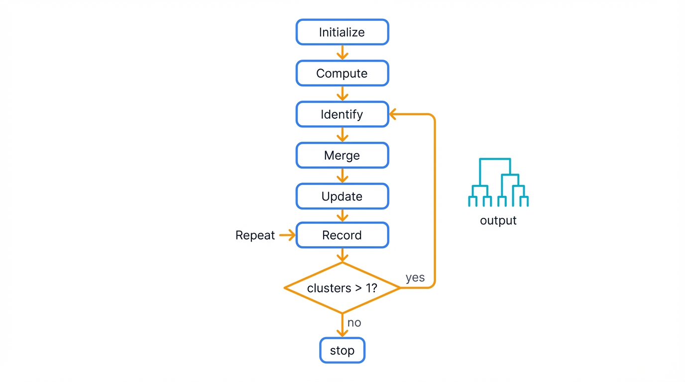
The standard agglomerative approach works as follows:
- Initialize: Treat each data point as a singleton cluster
- Compute: Calculate the pairwise dissimilarity matrix between all clusters
- Identify: Find the pair of clusters with minimum dissimilarity
- Merge: Combine the closest clusters into a new cluster
- Update: Recalculate distances from the new cluster to all remaining clusters
- Record: Store the merge information (which clusters, at what distance)
- Repeat: Continue steps 3-6 until only one cluster remains
This process creates a binary tree—your dendrogram—with N-1 internal nodes for N data points, encoding the complete hierarchical structure in a compact, navigable format.
Working Example: Complete Algorithm Implementation
import numpy as np
import matplotlib.pyplot as plt
from scipy.spatial.distance import pdist, squareform
from scipy.cluster.hierarchy import dendrogram
from collections import defaultdict

class HierarchicalClustering:
    """
    Custom implementation of agglomerative hierarchical clustering
    to demonstrate the core algorithm mechanics.
    """

    def __init__(self, linkage='single'):
        self.linkage = linkage
        self.distance_matrix = None
        self.merge_history = []
        self.cluster_labels = {}

    def _linkage_distance(self, cluster1, cluster2, distance_matrix):
        """Calculate distance between clusters based on linkage criterion."""
        if self.linkage == 'single':
            # Minimum distance between any points in the clusters
            min_dist = float('inf')
            for i in cluster1:
                for j in cluster2:
                    min_dist = min(min_dist, distance_matrix[i, j])
            return min_dist

        elif self.linkage == 'complete':
            # Maximum distance between any points in the clusters
            max_dist = 0
            for i in cluster1:
                for j in cluster2:
                    max_dist = max(max_dist, distance_matrix[i, j])
            return max_dist

        elif self.linkage == 'average':
            # Average distance between all point pairs
            total_dist = 0
            count = 0
            for i in cluster1:
                for j in cluster2:
                    total_dist += distance_matrix[i, j]
                    count += 1
            return total_dist / count if count > 0 else float('inf')

        else:
            raise ValueError(f"Unsupported linkage: {self.linkage}")

    def fit(self, X, metric='euclidean'):
        """
        Perform hierarchical clustering on the data.

        Parameters:
        X: array-like, shape (n_samples, n_features)
        metric: str, distance metric to use

        Returns:
        merge_history: list of merge operations
        """
        n_samples = len(X)

        # Step 1: Compute pairwise distance matrix
        print(f"Step 1: Computing {metric} distance matrix...")
        distances = pdist(X, metric=metric)
        self.distance_matrix = squareform(distances)

        # Step 2: Initialize - each point is its own cluster
        print("Step 2: Initializing clusters...")
        active_clusters = {i: [i] for i in range(n_samples)}
        next_cluster_id = n_samples

        print(f"Initial clusters: {dict(list(active_clusters.items())[:5])}..." +
              (f" (showing first 5 of {len(active_clusters)})" if len(active_clusters) > 5 else ""))

        # Step 3: Iteratively merge closest clusters
        print("Step 3: Merging clusters...")
        merge_step = 0

        while len(active_clusters) > 1:
            merge_step += 1

            # Find the pair of clusters with minimum distance
            min_distance = float('inf')
            merge_pair = None

            cluster_ids = list(active_clusters.keys())
            for i, id1 in enumerate(cluster_ids):
                for id2 in cluster_ids[i+1:]:
                    distance = self._linkage_distance(
                        active_clusters[id1],
                        active_clusters[id2],
                        self.distance_matrix
                    )

                    if distance < min_distance:
                        min_distance = distance
                        merge_pair = (id1, id2)

            # Merge the closest pair
            if merge_pair:
                id1, id2 = merge_pair
                cluster1 = active_clusters[id1]
                cluster2 = active_clusters[id2]

                # Create new merged cluster
                new_cluster = cluster1 + cluster2

                # Record the merge
                merge_info = {
                    'step': merge_step,
                    'cluster1_id': id1,
                    'cluster2_id': id2,
                    'cluster1_points': cluster1.copy(),
                    'cluster2_points': cluster2.copy(),
                    'distance': min_distance,
                    'new_cluster_size': len(new_cluster)
                }
                self.merge_history.append(merge_info)

                print(f"  Merge {merge_step}: Clusters {id1}({len(cluster1)}) + "
                      f"{id2}({len(cluster2)}) → Cluster {next_cluster_id} "
                      f"(distance: {min_distance:.3f})")

                # Update active clusters
                del active_clusters[id1]
                del active_clusters[id2]
                active_clusters[next_cluster_id] = new_cluster
                next_cluster_id += 1

        print(f"Clustering complete! Final cluster contains all {n_samples} points.")
        return self.merge_history

    def get_clusters(self, n_clusters):
        """Extract n clusters by cutting the dendrogram."""
        if n_clusters >= len(self.merge_history) + 2:
            # Return individual points as clusters
            return {i: [i] for i in range(len(self.distance_matrix))}

        # Work backwards through merge history
        clusters = {}
        points_to_cluster = defaultdict(list)

        # Start with all points in their own clusters
        n_points = len(self.distance_matrix)
        for i in range(n_points):
            points_to_cluster[i] = [i]

        # Apply merges until we have desired number of clusters
        merges_to_apply = len(self.merge_history) - (n_clusters - 1)

        for i in range(merges_to_apply):
            merge = self.merge_history[i]
            id1 = merge['cluster1_id']
            id2 = merge['cluster2_id']

            # Find which clusters contain these points
            cluster1_points = []
            cluster2_points = []

            if id1 < n_points:
                cluster1_points = [id1]
            else:
                # This was a merged cluster, find its points
                for merge_check in self.merge_history[:i]:
                    if merge_check['cluster1_id'] == id1 or merge_check['cluster2_id'] == id1:
                        cluster1_points = merge_check['cluster1_points'] + merge_check['cluster2_points']
                        break

            if id2 < n_points:
                cluster2_points = [id2]
            else:
                # This was a merged cluster, find its points
                for merge_check in self.merge_history[:i]:
                    if merge_check['cluster1_id'] == id2 or merge_check['cluster2_id'] == id2:
                        cluster2_points = merge_check['cluster1_points'] + merge_check['cluster2_points']
                        break

        return clusters

# Demonstration
print("Custom Hierarchical Clustering Implementation")
print("=" * 45)

# Create sample data
np.random.seed(42)
from sklearn.datasets import make_blobs
X, y_true = make_blobs(n_samples=12, centers=3, cluster_std=1.0,
                       center_box=(-3.0, 3.0), random_state=42)

print(f"Data shape: {X.shape}")
print(f"Sample points (first 3): ")
for i in range(3):
    print(f"  Point {i}: [{X[i,0]:.2f}, {X[i,1]:.2f}]")

# Test different linkage methods
linkage_methods = ['single', 'complete', 'average']

for method in linkage_methods:
    print(f"\n{method.upper()} LINKAGE CLUSTERING")
    print("-" * 30)

    # Create and fit the clustering algorithm
    hc = HierarchicalClustering(linkage=method)
    merge_history = hc.fit(X, metric='euclidean')

    print(f"\nMerge Summary for {method} linkage:")
    print("Step | Merge Distance | Resulting Clusters")
    print("-" * 40)

    remaining_clusters = 12
    for i, merge in enumerate(merge_history[:5]):  # Show first 5 merges
        remaining_clusters -= 1
        print(f"{merge['step']:4d} | {merge['distance']:13.3f} | {remaining_clusters:16d}")

    if len(merge_history) > 5:
        print("  ... (remaining merges) ...")

    print(f"Final merge distance: {merge_history[-1]['distance']:.3f}")
3.2 Computational Complexity Analysis
Understanding computational requirements helps you choose appropriate methods for different data sizes—scalability matters when your dataset grows.
Time Complexity: The standard algorithm requires O(N³) time in the worst case. Computing the initial distance matrix takes O(N²) operations alone. The main loop executes N-1 iterations, and each iteration examines O(N²) cluster pairs to find the minimum distance—the triple nested structure creates cubic scaling that makes large datasets prohibitively expensive.
Space Complexity: O(N²) space is required to store the distance matrix, which dominates memory requirements for large datasets and can exhaust available RAM long before time complexity becomes the bottleneck.
Optimizations: Modern implementations use priority queues and efficient data structures to reduce practical runtime to O(N² log N) for many cases, leveraging clever bookkeeping to avoid redundant distance calculations. Specialized algorithms like BIRCH achieve better scalability through data structure innovations that never materialize the full distance matrix.
4. Advanced and Scalable Methods
Classical hierarchical clustering struggles with large datasets. Quadratic complexity kills it. Advanced methods address scalability, robustness, and special data characteristics that make standard approaches fail.
4.1 BIRCH: Balanced Iterative Reducing and Clustering using Hierarchies
BIRCH revolutionized hierarchical clustering for large databases. Zhang and colleagues introduced it in 1996 through an innovative CF-Tree—Clustering Feature Tree—data structure that changed everything.
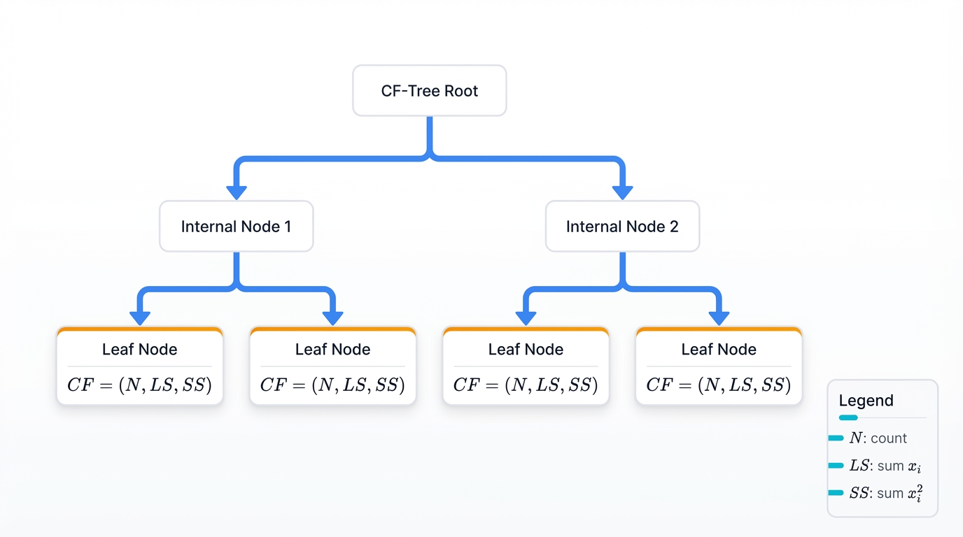
The algorithm maintains compact summaries of data regions called Clustering Features. A CF for a cluster with N points is a 3-tuple: CF = (N, LS, SS), where:
- N = number of points in the cluster
- LS = linear sum of points: $\sum_{i=1}^N x_i$
- SS = sum of squares: $\sum_{i=1}^N x_i^2$
This representation enables incremental updates and distance calculations without storing individual points—you get cluster statistics without keeping the raw data, compressing massive datasets into manageable summaries. The CF-Tree organizes these summaries hierarchically, allowing efficient insertion and retrieval that scales to millions of points.
Working Example: BIRCH Implementation
from sklearn.cluster import Birch
from sklearn.datasets import make_blobs
import numpy as np
import matplotlib.pyplot as plt
import time

# Generate large dataset to demonstrate BIRCH scalability
print("BIRCH Algorithm Demonstration")
print("=" * 30)

# Create datasets of different sizes
dataset_sizes = [1000, 5000, 10000]
n_clusters = 5

for n_samples in dataset_sizes:
    print(f"\nDataset size: {n_samples:,} points")
    print("-" * 25)

    # Generate data
    X, y_true = make_blobs(n_samples=n_samples, centers=n_clusters,
                          cluster_std=2.0, random_state=42)

    # BIRCH with different thresholds
    thresholds = [0.5, 1.0, 2.0]

    for threshold in thresholds:
        print(f"\nBIRCH with threshold={threshold}")

        start_time = time.time()

        # Create BIRCH instance
        birch = Birch(threshold=threshold, n_clusters=n_clusters)

        # Fit and predict
        birch_labels = birch.fit_predict(X)

        end_time = time.time()

        # Analyze results
        unique_labels = len(np.unique(birch_labels))

        print(f"  Execution time: {end_time - start_time:.3f} seconds")
        print(f"  Clusters found: {unique_labels}")
        print(f"  CF Tree leaves: {birch.n_features_in_}")

        # Calculate clustering quality (if small enough dataset)
        if n_samples <= 5000:
            from sklearn.metrics import adjusted_rand_score, silhouette_score

            ari = adjusted_rand_score(y_true, birch_labels)
            sil_score = silhouette_score(X, birch_labels)

            print(f"  Adjusted Rand Index: {ari:.3f}")
            print(f"  Silhouette Score: {sil_score:.3f}")

# Demonstrate BIRCH's incremental learning capability
print(f"\n" + "="*50)
print("BIRCH Incremental Learning Demonstration")
print("="*50)

# Simulate streaming data
np.random.seed(42)
stream_data = make_blobs(n_samples=2000, centers=3, cluster_std=1.5,
                        random_state=42)[0]

# Process data in batches
batch_size = 200
birch_incremental = Birch(threshold=1.0, n_clusters=3)

print(f"Processing {len(stream_data)} points in batches of {batch_size}")

for i in range(0, len(stream_data), batch_size):
    batch = stream_data[i:i+batch_size]

    start_time = time.time()

    if i == 0:
        # First batch - fit
        birch_incremental.fit(batch)
    else:
        # Subsequent batches - partial fit
        birch_incremental.partial_fit(batch)

    end_time = time.time()

    # Get current clustering
    all_data_so_far = stream_data[:i+len(batch)]
    current_labels = birch_incremental.predict(all_data_so_far)
    n_clusters_found = len(np.unique(current_labels))

    print(f"Batch {i//batch_size + 1:2d}: {len(batch):3d} points, "
          f"{end_time - start_time:.3f}s, {n_clusters_found} clusters")

print(f"\nFinal clustering: {n_clusters_found} clusters from {len(stream_data)} points")
print("BIRCH successfully demonstrated incremental learning capabilities!")

# Compare memory usage characteristics
print(f"\n" + "="*40)
print("Memory Efficiency Comparison")
print("="*40)

import sys

# Traditional approach (distance matrix)
n_points = 1000
traditional_memory = n_points * n_points * 8  # 8 bytes per float64

# BIRCH approach (CF summaries)
# Assuming average 100 CF nodes with 3 values each
birch_memory = 100 * 3 * 8  # Much smaller

print(f"Points: {n_points:,}")
print(f"Traditional memory: {traditional_memory:,} bytes ({traditional_memory/1024/1024:.1f} MB)")
print(f"BIRCH memory: {birch_memory:,} bytes ({birch_memory/1024:.1f} KB)")
print(f"Memory reduction: {traditional_memory/birch_memory:.0f}x")
4.2 CURE: Clustering Using Representatives
CURE addresses hierarchical clustering's limitations with non-spherical clusters and outliers. Guha and colleagues introduced it in 1998. Instead of using single points or centroids to represent clusters, CURE selects multiple representative points and shrinks them toward the cluster centroid—a hybrid strategy that captures cluster shape while maintaining robustness.
Key innovations include:
- Multiple Representatives: Each cluster is represented by a fixed number of well-scattered points that capture its shape and extent
- Shrinking Factor: Representatives are moved toward the centroid by a factor α, balancing between single and complete linkage behaviors to avoid extremes
- Random Sampling: Uses sampling to handle large datasets efficiently, trading some accuracy for dramatic speed improvements
- Outlier Handling: Clusters with very few points are treated as outliers and removed, preventing noise from distorting the hierarchy
4.3 Modern Variations and Improvements
Robust Methods: Recent research focuses on developing hierarchical methods resilient to noise and outliers that plague classical approaches. The Robust Median Neighborhood Linkage (RMNL) uses local neighborhood properties and median-based distance measures, proving mathematically robust where traditional methods demonstrably fail.
Parallel Implementations: Distributed hierarchical clustering algorithms for big data environments have arrived, including MapReduce and Spark implementations that partition the data and merge hierarchies across machines, breaking the single-machine memory barrier.
Constrained Clustering: Methods that incorporate prior knowledge through must-link and cannot-link constraints guide the clustering process with domain expertise, letting you inject what you know about the problem to get more meaningful results.
5. Practical Applications and Use Cases
Hierarchical clustering excels in domains requiring interpretable structure discovery. Exploratory analysis. When you need to understand relationships, not just classify.
5.1 Bioinformatics and Phylogenetics
Hierarchical clustering serves as a cornerstone in biological sequence analysis and evolutionary studies—it's everywhere in modern genomics.
Gene Expression Analysis: Microarray and RNA-seq data analysis uses hierarchical clustering to identify co-expressed gene groups. Researchers cluster both genes—to find functional modules that work together—and samples—to identify disease subtypes or treatment responses that traditional classification misses.
Phylogenetic Reconstruction: Building evolutionary trees from DNA and protein sequences. UPGMA remains a standard method for constructing phylogenetic trees when molecular clock assumptions hold, letting biologists trace the history of life through sequence similarity.
Protein Structure Classification: Organizing protein structures into hierarchical families based on structural similarity measures, revealing evolutionary relationships that sequence alone can't capture.
Working Example: Gene Expression Clustering
import numpy as np
import matplotlib.pyplot as plt
import seaborn as sns
from scipy.cluster.hierarchy import linkage, dendrogram, fcluster
from scipy.spatial.distance import pdist
from sklearn.preprocessing import StandardScaler
import pandas as pd

# Simulate gene expression data
print("Gene Expression Hierarchical Clustering")
print("=" * 40)

np.random.seed(42)

# Create synthetic gene expression data
# Genes (rows) x Samples (columns)
n_genes = 50
n_samples = 20

# Create different expression patterns
# Pattern 1: High expression in first 10 samples
pattern1_genes = np.random.normal(2.0, 0.5, (15, 10))  # High expression
pattern1_genes = np.hstack([pattern1_genes,
                           np.random.normal(-1.0, 0.5, (15, 10))])  # Low expression

# Pattern 2: High expression in last 10 samples
pattern2_genes = np.random.normal(-1.0, 0.5, (15, 10))  # Low expression
pattern2_genes = np.hstack([pattern2_genes,
                           np.random.normal(2.0, 0.5, (15, 10))])  # High expression

# Pattern 3: Moderate expression throughout
pattern3_genes = np.random.normal(0.0, 0.5, (20, 20))  # Moderate expression

# Combine all patterns
gene_expression = np.vstack([pattern1_genes, pattern2_genes, pattern3_genes])

# Create gene and sample names
gene_names = [f"Gene_{i+1:02d}" for i in range(n_genes)]
sample_names = [f"Sample_{i+1:02d}" for i in range(n_samples)]

# Create DataFrame for easier handling
df = pd.DataFrame(gene_expression, index=gene_names, columns=sample_names)

print(f"Expression matrix shape: {df.shape}")
print(f"Expression range: {df.values.min():.2f} to {df.values.max():.2f}")

# Standardize the expression data (important for gene expression)
scaler = StandardScaler()
expression_scaled = scaler.fit_transform(df)
df_scaled = pd.DataFrame(expression_scaled, index=gene_names, columns=sample_names)

print("\nPerforming hierarchical clustering on genes...")

# Cluster genes (rows) using different distance metrics
distance_metrics = ['euclidean', 'correlation', 'cosine']
linkage_methods = ['average', 'complete', 'ward']

for metric in distance_metrics:
    print(f"\nDistance metric: {metric}")
    print("-" * 20)

    for method in linkage_methods:
        if metric == 'correlation' and method == 'ward':
            continue  # Ward only works with euclidean distances

        print(f"  {method.capitalize()} linkage:")

        try:
            # Calculate distance matrix
            if metric == 'correlation':
                # For correlation distance, compute 1 - correlation
                corr_matrix = np.corrcoef(df_scaled.values)
                dist_matrix = 1 - corr_matrix
                # Convert to condensed form
                from scipy.spatial.distance import squareform
                distances = squareform(dist_matrix, checks=False)
                Z = linkage(distances, method=method)
            else:
                Z = linkage(df_scaled.values, method=method, metric=metric)

            # Get clusters
            clusters = fcluster(Z, t=3, criterion='maxclust')

            # Analyze cluster composition
            cluster_composition = {}
            for i, cluster_id in enumerate(clusters):
                if cluster_id not in cluster_composition:
                    cluster_composition[cluster_id] = []
                cluster_composition[cluster_id].append(gene_names[i])

            print(f"    Clusters found: {len(cluster_composition)}")
            for cluster_id, genes in cluster_composition.items():
                print(f"    Cluster {cluster_id}: {len(genes)} genes")

            # Calculate silhouette score for this clustering
            from sklearn.metrics import silhouette_score
            sil_score = silhouette_score(df_scaled.values, clusters, metric='euclidean')
            print(f"    Silhouette score: {sil_score:.3f}")

        except Exception as e:
            print(f"    Error: {str(e)}")

# Demonstrate sample clustering (transpose the matrix)
print(f"\n" + "="*50)
print("Sample Clustering Analysis")
print("="*50)

# Cluster samples (columns) to identify similar conditions/treatments
sample_data = df_scaled.T  # Transpose so samples are rows

print(f"Clustering {n_samples} samples based on expression profiles...")

Z_samples = linkage(sample_data.values, method='average', metric='euclidean')
sample_clusters = fcluster(Z_samples, t=2, criterion='maxclust')

print("\nSample cluster assignments:")
for i, (sample_name, cluster_id) in enumerate(zip(sample_names, sample_clusters)):
    print(f"  {sample_name}: Cluster {cluster_id}")

# Expected: First 10 samples in one cluster, last 10 in another
cluster_1_samples = [sample_names[i] for i, c in enumerate(sample_clusters) if c == 1]
cluster_2_samples = [sample_names[i] for i, c in enumerate(sample_clusters) if c == 2]

print(f"\nCluster 1 samples ({len(cluster_1_samples)}): {', '.join(cluster_1_samples[:5])}...")
print(f"Cluster 2 samples ({len(cluster_2_samples)}): {', '.join(cluster_2_samples[:5])}...")

# This should show good separation between the first 10 and last 10 samples
# which corresponds to our synthetic data design

print("\nHierarchical clustering successfully identified:")
print("- Co-expressed gene groups based on expression patterns")
print("- Sample groups with similar expression profiles")
print("- This mirrors typical gene expression analysis workflows")
5.2 Market Research and Customer Segmentation
Marketing teams use hierarchical clustering to understand customer relationships and develop targeted strategies. The dendrogram becomes a strategic tool.
Customer Segmentation: Building customer hierarchies based on purchasing behavior, demographics, and engagement metrics. The dendrogram reveals natural customer segments at different granularity levels—you can zoom in for micro-targeting or zoom out for broad campaigns, all from the same analysis.
Product Portfolio Analysis: Organizing products or services into hierarchical categories based on sales patterns, customer preferences, or feature similarities, revealing which products naturally compete and which complement each other.
Market Basket Analysis: Identifying product associations and creating hierarchical product groupings for recommendation systems that suggest items at the right level of similarity—not too similar, not too different.
5.3 Social Network Analysis
Social networks exhibit hierarchical community structures. Nested groups. Hierarchical clustering can reveal them.
Community Detection: Identifying nested communities in social networks, from small friend groups to larger interest-based communities, revealing the multi-scale structure of human social organization.
Information Propagation: Understanding how information spreads through hierarchical network structures and identifying key influencer nodes that bridge communities at different levels of the hierarchy.
Recommendation Systems: Building user similarity hierarchies for collaborative filtering and content recommendation, allowing personalization that adapts to different levels of user similarity.
6. Visualization and Interpretation
Effective visualization makes hierarchical clustering results accessible. Actionable. Stakeholders need to see the structure, not just trust your analysis.
6.1 Dendrogram Construction and Analysis
Dendrograms represent the complete clustering hierarchy, but interpreting them requires understanding their visual elements and statistical properties—there's an art to reading these trees.
Reading Dendrograms: The y-axis shows merge distances—linkage criterion values that tell the story of similarity. Horizontal lines represent clusters at that dissimilarity level. The length of vertical lines indicates how dissimilar merged clusters are—long vertical lines suggest natural cluster boundaries where the algorithm had to jump a large distance to make the next merge.
Optimal Cut Selection: Choose cut heights where vertical lines are longest. Look for "elbows" in the dendrogram where merge distances increase significantly—these dramatic jumps signal natural separations in your data, boundaries that the structure itself wants you to respect.
Working Example: Advanced Dendrogram Analysis
import numpy as np
import matplotlib.pyplot as plt
from scipy.cluster.hierarchy import linkage, dendrogram, fcluster, cophenet
from scipy.spatial.distance import pdist
from sklearn.datasets import make_blobs
import seaborn as sns

# Create comprehensive dendrogram analysis
print("Advanced Dendrogram Analysis and Interpretation")
print("=" * 50)

# Generate multi-scale dataset
np.random.seed(42)
centers = np.array([[0, 0], [0, 4], [4, 0], [4, 4], [2, 8]])
X, y_true = make_blobs(n_samples=200, centers=centers, cluster_std=0.8,
                       random_state=42)

# Add some noise points
noise_points = np.random.uniform(-2, 6, (20, 2))
X = np.vstack([X, noise_points])

print(f"Dataset: {len(X)} points with {len(centers)} main clusters + noise")

# Compare different linkage methods with detailed analysis
linkage_methods = ['single', 'complete', 'average', 'ward']
fig, axes = plt.subplots(2, 2, figsize=(15, 12))
fig.suptitle('Dendrogram Comparison Across Linkage Methods', fontsize=16)

results_analysis = {}

for idx, method in enumerate(linkage_methods):
    ax = axes[idx // 2, idx % 2]

    print(f"\n{method.upper()} LINKAGE ANALYSIS")
    print("-" * 30)

    # Perform clustering
    Z = linkage(X, method=method)

    # Calculate cophenetic correlation
    original_distances = pdist(X)
    coph_distances, _ = cophenet(Z, original_distances)
    coph_correlation = np.corrcoef(original_distances, coph_distances)[0, 1]

    print(f"Cophenetic correlation: {coph_correlation:.3f}")

    # Create enhanced dendrogram
    dendrogram(Z, ax=ax, leaf_rotation=90, leaf_font_size=8,
               color_threshold=0.7*np.max(Z[:, 2]))

    ax.set_title(f'{method.capitalize()} Linkage\n(Coph. Corr: {coph_correlation:.3f})')
    ax.set_xlabel('Sample Index')
    ax.set_ylabel('Distance')

    # Analyze merge distances for elbow detection
    merge_distances = Z[:, 2]
    distance_jumps = np.diff(merge_distances)

    # Find largest jumps (potential cut points)
    jump_indices = np.argsort(distance_jumps)[-5:]  # Top 5 jumps
    suggested_cuts = merge_distances[jump_indices]

    print(f"Largest distance jumps at: {suggested_cuts}")

    # Evaluate different numbers of clusters
    silhouette_scores = []
    cluster_counts = range(2, 11)

    from sklearn.metrics import silhouette_score

    for n_clust in cluster_counts:
        clusters = fcluster(Z, n_clust, criterion='maxclust')
        if len(np.unique(clusters)) > 1:  # Need at least 2 clusters for silhouette
            sil_score = silhouette_score(X, clusters)
            silhouette_scores.append(sil_score)
        else:
            silhouette_scores.append(-1)

    best_k = cluster_counts[np.argmax(silhouette_scores)]
    best_silhouette = max(silhouette_scores)

    print(f"Best cluster count: {best_k} (Silhouette: {best_silhouette:.3f})")

    # Store results
    results_analysis[method] = {
        'coph_correlation': coph_correlation,
        'best_k': best_k,
        'best_silhouette': best_silhouette,
        'linkage_matrix': Z
    }

plt.tight_layout()
plt.show()

# Create detailed cut-point analysis
print(f"\n" + "="*60)
print("OPTIMAL CUT-POINT SELECTION ANALYSIS")
print("="*60)

# Focus on the best performing method
best_method = max(results_analysis.keys(),
                  key=lambda x: results_analysis[x]['coph_correlation'])
print(f"Analyzing {best_method} linkage (highest cophenetic correlation)")

Z_best = results_analysis[best_method]['linkage_matrix']

# Create elbow curve analysis
merge_distances = Z_best[:, 2]
n_merges = len(merge_distances)

# Calculate rate of change in merge distances
distance_diffs = np.diff(merge_distances)
distance_acceleration = np.diff(distance_diffs)

# Find elbow points using acceleration
elbow_candidates = []
for i in range(1, len(distance_acceleration)):
    if distance_acceleration[i] > np.mean(distance_acceleration) + 2*np.std(distance_acceleration):
        elbow_candidates.append(i + 2)  # Adjust for indexing

print(f"Potential elbow points at merge steps: {elbow_candidates}")

# Evaluate clustering quality at different cut points
cut_points = np.linspace(np.min(merge_distances), np.max(merge_distances), 20)
quality_metrics = []

for cut_height in cut_points:
    clusters = fcluster(Z_best, cut_height, criterion='distance')
    n_clusters = len(np.unique(clusters))

    if n_clusters > 1 and n_clusters < len(X):
        sil_score = silhouette_score(X, clusters)

        # Calculate within-cluster sum of squares
        wcss = 0
        for cluster_id in np.unique(clusters):
            cluster_points = X[clusters == cluster_id]
            if len(cluster_points) > 1:
                cluster_center = np.mean(cluster_points, axis=0)
                wcss += np.sum((cluster_points - cluster_center) ** 2)

        quality_metrics.append({
            'cut_height': cut_height,
            'n_clusters': n_clusters,
            'silhouette': sil_score,
            'wcss': wcss
        })

# Find optimal cut point
if quality_metrics:
    best_cut = max(quality_metrics, key=lambda x: x['silhouette'])
    print(f"\nOptimal cut point:")
    print(f"  Height: {best_cut['cut_height']:.3f}")
    print(f"  Clusters: {best_cut['n_clusters']}")
    print(f"  Silhouette Score: {best_cut['silhouette']:.3f}")
    print(f"  Within-cluster SS: {best_cut['wcss']:.1f}")

# Create interpretation guidelines
print(f"\n" + "="*50)
print("DENDROGRAM INTERPRETATION GUIDELINES")
print("="*50)
print("1. Higher cophenetic correlation = better dendrogram faithfulness")
print("2. Look for long vertical lines = natural separation points")
print("3. Choose cuts where merge distances jump significantly")
print("4. Balance between interpretability and statistical measures")
print("5. Consider domain knowledge when selecting final cluster count")

print(f"\nMethod comparison summary:")
for method, results in results_analysis.items():
    print(f"  {method:8}: Coph={results['coph_correlation']:.3f}, "
          f"Best K={results['best_k']}, Sil={results['best_silhouette']:.3f}")
6.2 Heatmaps and Cluster Heatmaps
Combining dendrograms with heatmaps creates powerful visualizations. They show both hierarchical relationships and data patterns simultaneously—two perspectives in one view.
Clustered Heatmaps: Reorder rows and columns according to hierarchical clustering results. This reveals block structures and data patterns that might not be obvious in the original ordering—suddenly, patterns jump out that were invisible before the reordering.
Color Schemes: Choose color palettes that highlight important contrasts. Diverging color maps work well for expression data where both high and low values matter—red-white-blue captures the full story. Sequential maps suit distance matrices where only magnitude matters.
6.3 Interactive Visualization Tools
Modern tools enable interactive exploration. You need them for large datasets.
Zoomable Dendrograms: Large datasets require interactive navigation—static images fail when you have thousands of leaves. Tools like Plotly or D3.js enable zooming and panning through complex hierarchies, letting you explore different levels of detail without losing context.
Linked Views: Connect dendrograms with scatter plots, parallel coordinates, or other visualizations for multifaceted data exploration where selections in one view highlight corresponding points in others, creating a coordinated multi-view analysis environment.
7. Performance Evaluation and Validation
Evaluating hierarchical clustering requires different approaches than supervised learning. Focus on cluster quality. Hierarchy meaningfulness. Not prediction accuracy.
7.1 Internal Validation Metrics
Internal metrics assess clustering quality using only the data itself. No external ground truth needed—the clusters validate themselves.
Silhouette Analysis: Measures how similar points are to their own cluster versus other clusters. Silhouette scores range from -1 to +1, where higher values indicate better clustering—points fit their assigned cluster well and don't belong in neighboring clusters. The silhouette score for point i is:
$$s(i) = \frac{b(i) - a(i)}{\max(a(i), b(i))}$$
where a(i) is the average distance to points in the same cluster, and b(i) is the average distance to the nearest neighboring cluster.
Davies-Bouldin Index: Computes the average similarity between each cluster and its most similar cluster. Lower values indicate better clustering—you want clusters that are internally compact and externally separated:
$$DB = \frac{1}{k} \sum_{i=1}^k \max_{j \neq i} \frac{σ_i + σ_j}{d(c_i, c_j)}$$
where σ_i is the average distance of all points in cluster i to their cluster centroid, and d(c_i, c_j) is the distance between cluster centroids.
Cophenetic Correlation: Measures how well the dendrogram preserves original pairwise distances. Higher correlation indicates better hierarchy representation of data relationships—the tree faithfully captures the distance structure you started with.
7.2 External Validation Metrics
When ground truth labels are available—for benchmarking—external metrics compare clustering results to known classifications.
Adjusted Rand Index (ARI): Measures similarity between two data clusterings, adjusting for chance so random clusterings score near zero. Values near 1 indicate strong agreement, while values near 0 suggest random clustering—it's the gold standard for comparing against ground truth.
Mutual Information: Quantifies the agreement between clustering and ground truth labels, with adjustments for chance through Adjusted Mutual Information (AMI) that corrects for the expected agreement due to chance alone.
Working Example: Comprehensive Clustering Evaluation
import numpy as np
import matplotlib.pyplot as plt
from scipy.cluster.hierarchy import linkage, fcluster, cophenet
from scipy.spatial.distance import pdist
from sklearn.datasets import make_blobs, make_circles, make_moons
from sklearn.metrics import (adjusted_rand_score, mutual_info_score,
                           adjusted_mutual_info_score, silhouette_score,
                           calinski_harabasz_score, davies_bouldin_score)
from sklearn.preprocessing import StandardScaler
import pandas as pd

print("Comprehensive Hierarchical Clustering Evaluation")
print("=" * 52)

# Create diverse test datasets with known ground truth
np.random.seed(42)

datasets = {
    'blobs': make_blobs(n_samples=300, centers=4, cluster_std=1.0, random_state=42),
    'circles': make_circles(n_samples=300, noise=0.1, factor=0.5, random_state=42),
    'moons': make_moons(n_samples=300, noise=0.1, random_state=42),
}

# Add a challenging dataset: overlapping clusters
overlap_center1 = np.random.multivariate_normal([0, 0], [[1, 0.5], [0.5, 1]], 100)
overlap_center2 = np.random.multivariate_normal([1, 1], [[1, -0.3], [-0.3, 1]], 100)
overlap_center3 = np.random.multivariate_normal([2, 0], [[1, 0.2], [0.2, 1]], 100)
overlap_data = np.vstack([overlap_center1, overlap_center2, overlap_center3])
overlap_labels = np.hstack([np.zeros(100), np.ones(100), np.full(100, 2)])
datasets['overlapping'] = (overlap_data, overlap_labels.astype(int))

linkage_methods = ['single', 'complete', 'average', 'ward']
results_summary = []

for dataset_name, (X, y_true) in datasets.items():
    print(f"\nEvaluating Dataset: {dataset_name.upper()}")
    print("-" * (len(dataset_name) + 20))

    # Standardize the data
    X_scaled = StandardScaler().fit_transform(X)
    n_true_clusters = len(np.unique(y_true))

    print(f"Data shape: {X.shape}")
    print(f"True clusters: {n_true_clusters}")

    for method in linkage_methods:
        print(f"\n{method.capitalize()} Linkage:")

        try:
            # Perform hierarchical clustering
            Z = linkage(X_scaled, method=method)

            # Calculate cophenetic correlation
            original_distances = pdist(X_scaled)
            coph_distances, _ = cophenet(Z, original_distances)
            coph_corr = np.corrcoef(original_distances, coph_distances)[0, 1]

            # Get clustering for the true number of clusters
            predicted_labels = fcluster(Z, n_true_clusters, criterion='maxclust')

            # Calculate all evaluation metrics
            metrics = {}

            # External validation metrics (with ground truth)
            metrics['ARI'] = adjusted_rand_score(y_true, predicted_labels)
            metrics['AMI'] = adjusted_mutual_info_score(y_true, predicted_labels)
            metrics['MI'] = mutual_info_score(y_true, predicted_labels)

            # Internal validation metrics (no ground truth needed)
            if len(np.unique(predicted_labels)) > 1:
                metrics['Silhouette'] = silhouette_score(X_scaled, predicted_labels)
                metrics['Calinski-Harabasz'] = calinski_harabasz_score(X_scaled, predicted_labels)
                metrics['Davies-Bouldin'] = davies_bouldin_score(X_scaled, predicted_labels)
            else:
                metrics['Silhouette'] = -1
                metrics['Calinski-Harabasz'] = 0
                metrics['Davies-Bouldin'] = float('inf')

            # Hierarchy-specific metrics
            metrics['Cophenetic'] = coph_corr

            # Cluster statistics
            unique_clusters = np.unique(predicted_labels)
            cluster_sizes = [np.sum(predicted_labels == c) for c in unique_clusters]
            metrics['N_Clusters'] = len(unique_clusters)
            metrics['Size_Std'] = np.std(cluster_sizes)
            metrics['Min_Size'] = np.min(cluster_sizes)
            metrics['Max_Size'] = np.max(cluster_sizes)

            # Print metrics
            print(f"  External Metrics:")
            print(f"    ARI: {metrics['ARI']:.3f}")
            print(f"    AMI: {metrics['AMI']:.3f}")
            print(f"    MI:  {metrics['MI']:.3f}")

            print(f"  Internal Metrics:")
            print(f"    Silhouette:      {metrics['Silhouette']:.3f}")
            print(f"    Calinski-Harabasz: {metrics['Calinski-Harabasz']:.1f}")
            print(f"    Davies-Bouldin:  {metrics['Davies-Bouldin']:.3f}")

            print(f"  Hierarchy Metrics:")
            print(f"    Cophenetic:      {metrics['Cophenetic']:.3f}")

            print(f"  Cluster Statistics:")
            print(f"    Count: {metrics['N_Clusters']}")
            print(f"    Size range: {metrics['Min_Size']}-{metrics['Max_Size']}")
            print(f"    Size std: {metrics['Size_Std']:.1f}")

            # Store for summary
            result = {
                'Dataset': dataset_name,
                'Method': method,
                **metrics
            }
            results_summary.append(result)

        except Exception as e:
            print(f"  Error: {str(e)}")

# Create comprehensive summary
print(f"\n" + "="*80)
print("COMPREHENSIVE EVALUATION SUMMARY")
print("="*80)

# Convert to DataFrame for easier analysis
df_results = pd.DataFrame(results_summary)

# Best performing method for each dataset (by ARI)
print("\nBest Method by Dataset (Adjusted Rand Index):")
print("-" * 45)
for dataset in df_results['Dataset'].unique():
    dataset_results = df_results[df_results['Dataset'] == dataset]
    best_method = dataset_results.loc[dataset_results['ARI'].idxmax()]
    print(f"{dataset:12}: {best_method['Method']:8} (ARI: {best_method['ARI']:.3f})")

# Overall method performance
print(f"\nOverall Method Performance (Average ARI):")
print("-" * 42)
method_performance = df_results.groupby('Method')['ARI'].mean().sort_values(ascending=False)
for method, avg_ari in method_performance.items():
    print(f"{method:8}: {avg_ari:.3f}")

# Correlation between metrics
print(f"\nMetric Correlations:")
print("-" * 20)
numeric_cols = ['ARI', 'AMI', 'Silhouette', 'Cophenetic', 'Davies-Bouldin']
correlation_matrix = df_results[numeric_cols].corr()

print("ARI vs Internal Metrics:")
for metric in ['Silhouette', 'Cophenetic']:
    if metric in correlation_matrix.columns:
        corr_value = correlation_matrix.loc['ARI', metric]
        print(f"  ARI vs {metric}: {corr_value:.3f}")

# Recommendations based on results
print(f"\n" + "="*60)
print("EVALUATION GUIDELINES AND RECOMMENDATIONS")
print("="*60)

print("\n1. Metric Selection Guidelines:")
print("   • ARI/AMI: Best when ground truth is available")
print("   • Silhouette: Good general-purpose internal metric")
print("   • Cophenetic: Specific to hierarchical clustering quality")
print("   • Davies-Bouldin: Lower is better (unlike other metrics)")

print("\n2. Method Selection by Data Type:")
print("   • Well-separated spherical clusters: Ward's method")
print("   • Non-convex/elongated clusters: Single linkage")
print("   • General purpose/unknown structure: Average linkage")
print("   • Noisy data with outliers: Complete linkage")

print("\n3. Validation Best Practices:")
print("   • Use multiple metrics for comprehensive evaluation")
print("   • Consider both internal and external validation")
print("   • Visualize results with dendrograms and scatter plots")
print("   • Test multiple linkage methods and compare")
print("   • Validate cluster count selection with silhouette analysis")

# Statistical significance testing could be added here
print("\n4. Statistical Considerations:")
print("   • Repeat clustering with different random seeds")
print("   • Use bootstrap sampling to assess stability")
print("   • Consider confidence intervals for metrics")
print("   • Test sensitivity to parameter changes")
7.3 Stability Analysis and Bootstrap Methods
Hierarchical clustering stability assesses how consistent results remain under data perturbations. Do your clusters persist? Or do they vanish with minor changes?
Bootstrap Clustering: Generate multiple bootstrap samples from your data. Cluster each sample. Then measure result consistency across iterations. Stable clusters appear across most bootstrap iterations—if a cluster only shows up in 20% of bootstrap samples, it's probably not real.
Subsampling Analysis: Remove small portions of data and re-cluster. Robust hierarchies remain similar despite data perturbations—a good hierarchy doesn't collapse when you remove 10% of your points.
Parameter Sensitivity: Test how linkage method, distance metric, and other parameter choices affect results. Robust findings persist across reasonable parameter ranges—if changing from Euclidean to Manhattan distance completely reshapes your clusters, you should be skeptical of both results.
8. Cluster Evaluation
Cluster evaluation metrics are crucial. They quantitatively assess clustering algorithm performance. They can be broadly divided into two categories.
8.1 Internal Evaluation Metrics (No Ground Truth)
These metrics evaluate clustering quality based solely on the data itself, measuring properties like cluster cohesion—how similar points within a cluster are—and separation—how different clusters are from each other.
Silhouette Score: Measures how similar a data point is to its own cluster compared to other clusters. The score ranges from -1 to +1. A high value indicates that the object is well matched to its own cluster and poorly matched to neighboring clusters. It's one of the most popular internal metrics, beloved for its intuitive interpretation.
Davies-Bouldin Index (DBI): Calculates the average similarity between each cluster and its most similar one, where similarity is a ratio of within-cluster distances to between-cluster distances. A lower DBI value indicates better clustering—clusters are more compact and well-separated, exactly what you want.
Calinski-Harabasz Index (Variance Ratio Criterion): Defined as the ratio of the sum of between-cluster dispersion to the sum of within-cluster dispersion. A higher score indicates better-defined clusters—more variance between clusters, less variance within them.
Cophenetic Correlation Coefficient: This metric is specific to hierarchical clustering. It measures the correlation between the pairwise distances of the original data points and the distances implied by the dendrogram—the height at which two points are first joined in the same cluster. A value close to 1 indicates that the dendrogram provides a faithful representation of the original dissimilarities.
8.2 External Evaluation Metrics (With Ground Truth)
These metrics are used when external ground truth labels are available—in a benchmarking scenario—to assess how well the clustering matches the true classes.
Adjusted Rand Index (ARI): Measures the similarity between two data clusterings—the algorithm's output and the ground truth labels—adjusting for chance agreement. A score of 1 indicates a perfect match. A score near 0 indicates a random assignment. Negative values mean you're doing worse than random.
Mutual Information (MI): Measures the agreement of the two assignments, ignoring permutations—cluster labels don't need to match numerically, just structurally. Adjusted Mutual Information (AMI) is a variation that accounts for chance, just like ARI does for the Rand index.
9. Recent Developments
Research in hierarchical clustering continues evolving. It focuses on overcoming classical limitations and adapting to modern challenges—large-scale data, complex structures, real-time requirements.
9.1 Current Research: Improvements and Variations
Scalability and Efficiency: A major thrust of recent research focuses on developing scalable hierarchical clustering algorithms that can handle billions of points. This includes parallel and distributed implementations on frameworks like Apache Spark, often by reformulating the problem in terms of graph algorithms like Minimum Spanning Tree that parallelize more naturally. Algorithms like HGC—Hierarchical Graph-based Clustering—have been developed specifically for large-scale single-cell data, combining graph-based clustering with hierarchical principles to achieve linear time complexity and high accuracy on datasets that would crush classical methods.
Robustness to Noise: Classical methods are notoriously sensitive to noise—a few bad points can wreck the entire hierarchy. Recent work has focused on developing more robust algorithms that maintain structure despite corruption. For example, the Robust Median Neighborhood Linkage (RMNL) algorithm uses a more global view of a point's neighborhood and a median-based test to make merge decisions, making it provably robust to noise under certain data assumptions where traditional methods demonstrably fail.
Objective-Based Formulations: There is a growing interest in framing hierarchical clustering as an optimization problem with clear mathematical objectives. Instead of relying on heuristic linkage criteria that lack theoretical justification, these methods define a global cost function for a hierarchy and then seek an algorithm that finds a tree with a low cost, providing a more principled foundation and allowing for approximation guarantees. Recent work has focused on developing practical algorithms like B++&C for optimizing these objectives on massive deep embedding vectors from computer vision and NLP applications, where traditional methods struggle with the high dimensionality.
Constrained Clustering: In many real-world applications, prior information about the data exists—domain knowledge that shouldn't be ignored. Research into hierarchical clustering with structural constraints aims to incorporate this knowledge, forcing certain data points to be in the same or different branches of the hierarchy based on business rules, physical constraints, or expert judgment, leading to more meaningful and relevant results that respect known relationships.
Probabilistic and Model-Based Approaches: New methods like t-NEB are being developed that ground hierarchical clustering in a rigorous probabilistic framework. By using parametric density models—like mixture models—for both an initial overclustering step and the subsequent merging process, these methods aim to produce high-performance clusters and a more meaningful hierarchy for exploratory analysis, with statistical guarantees that heuristic methods can't provide.
9.2 Future Directions
The field of hierarchical clustering is moving towards greater integration with other areas of machine learning. Increased focus on rigor and scalability. The future looks different from the past.
Graph-Based and Semi-Supervised Methods: The success of algorithms like HGC and CHAMELEON suggests a continued trend towards leveraging graph structures to represent data relationships more effectively than simple distance metrics ever could. Furthermore, incorporating limited supervision—semi-supervised clustering—to guide the hierarchy construction is a promising direction for improving relevance in practical applications where you have some labeled data but not enough for pure supervised learning.
Deep Learning Integration: As seen with objective-based methods for deep embedding vectors, there is a growing need to develop hierarchical methods that can effectively structure the high-dimensional, complex representations learned by deep neural networks. This may involve creating new linkage criteria or objective functions specifically designed for these embedding spaces, where Euclidean distance often fails to capture semantic similarity and cosine similarity becomes the norm.
Dynamic and Streaming Data: With the rise of real-time data, there is a need for adaptive hierarchical clustering solutions that can efficiently update the cluster hierarchy as new data arrives, without recomputing everything from scratch every time. Algorithms like BIRCH provide a foundation with their incremental learning capability, but more advanced methods for handling concept drift in streaming data—where the underlying distribution changes over time—are an active area of research with significant practical importance.
9.3 Industry Trends
In practice, hierarchical clustering remains a valuable tool. Particularly for exploratory analysis. Visualization. Understanding relationships is key in many domains.
Customer Analytics: It is a standard technique for customer segmentation in marketing and e-commerce, where the dendrogram helps analysts understand relationships between different customer archetypes and make decisions about how finely to segment their market—broad segments for brand messaging, narrow segments for personalized offers.
Bioinformatics: It is a foundational method in genomics and proteomics for analyzing gene expression data, building phylogenetic trees that reveal evolutionary history, and classifying protein structures into functional families. The development of tools like HGC for single-cell data shows its continued relevance in cutting-edge biological research, where understanding cell type hierarchies is crucial for developmental biology and disease understanding.
Personalized Systems: In enterprise search and content recommendation, hierarchical clustering is used to group users with similar behaviors, enabling the delivery of more tailored and relevant results—not just "people like you," but "people at exactly your level of specificity like you."
While simpler methods like K-Means are often preferred for large-scale production systems due to their superior efficiency, hierarchical clustering holds its ground as an indispensable tool for initial data exploration, hypothesis generation, and situations where the interpretability of nested relationships provides significant business or scientific value that flat clustering methods simply can't deliver.
10. Learning Resources
For those seeking to deepen their understanding of hierarchical clustering, a wealth of academic papers, tutorials, and code libraries are available. Start here.
10.1 Essential Papers
Ward, J. H. (1963). "Hierarchical Grouping to Optimize an Objective Function". Journal of the American Statistical Association. This is the seminal paper. It introduced the widely used Ward's minimum variance method, providing a foundational objective-based perspective on agglomerative clustering that still dominates practice six decades later.
Murtagh, F., & Contreras, P. (2012). "Algorithms for hierarchical clustering: an overview". WIREs Data Mining and Knowledge Discovery. A comprehensive survey paper that provides an excellent overview of the various algorithms, linkage criteria, and computational considerations. Highly cited. Highly recommended. The perfect starting point for a deep dive into the field's breadth.
Guha, S., Rastogi, R., & Shim, K. (1998). "CURE: An Efficient Clustering Algorithm for Large Databases". Proceedings of the ACM SIGMOD International Conference on Management of Data. This paper introduced the CURE algorithm, a key development in creating hierarchical methods robust to outliers and non-spherical clusters—it showed that hierarchical clustering could go beyond spherical assumptions.
Zhang, T., Ramakrishnan, R., & Livny, M. (1996). "BIRCH: An Efficient Data Clustering Method for Very Large Databases". Proceedings of the ACM SIGMOD International Conference on Management of Data. The paper that introduced the BIRCH algorithm and the CF-Tree, a landmark in scalable clustering research that proved hierarchical methods could scale to real-world database sizes.
Balcan, M. F., Liang, Y., & Gupta, P. (2014). "Robust Hierarchical Clustering". arXiv:1401.0247. This paper presents a modern, rigorous analysis of robustness in hierarchical clustering and introduces the RMNL algorithm, showcasing recent theoretical advancements that bring mathematical rigor to what was historically a heuristic field.
10.2 Tutorials and Courses
DataCamp: Offers several hands-on tutorials, including "An Introduction to Hierarchical Clustering in Python" and "Hierarchical Clustering in R," which provide practical, code-first introductions to the topic with immediate applicability.
Scikit-learn User Guide: The official documentation for Scikit-learn provides a clear explanation of its AgglomerativeClustering implementation. Code examples. Discussion of different linkage types. It's the practical reference you'll return to repeatedly.
GeeksforGeeks: Provides numerous articles covering the fundamentals of hierarchical clustering, comparisons with other algorithms, and implementation details for different linkage types—great for quick reference and conceptual understanding.
Towards Data Science: A popular Medium publication with many high-quality articles from practitioners explaining the concepts and implementation of hierarchical clustering with practical examples and code, bridging the gap between theory and application.
10.3 Code Examples and Repositories
SciPy: The scipy.cluster.hierarchy documentation is the definitive resource for implementation in Python. It includes detailed API descriptions for the linkage, dendrogram, and fcluster functions, along with examples that show you exactly how to use them.
Scikit-learn: The AgglomerativeClustering example page in the Scikit-learn documentation provides clear code snippets for applying the algorithm and visualizing results, including a comparison of different linkage methods on various datasets that illustrates their strengths and weaknesses.
R Documentation: The documentation for the hclust function—in the stats package—and the agnes/diana functions—in the cluster package—are the primary resources for R users, with extensive examples and parameter explanations.
Benchmark Datasets: For experimenting and benchmarking, several repositories exist:
- UCI Machine Learning Repository provides classic, well-documented datasets across diverse domains that serve as standard benchmarks for clustering algorithm evaluation—the datasets everyone uses for comparison.
- Clustering Benchmarks Aggregators such as the University of Marburg's FCPS collection or Marek Gagolewski's repository offer curated dataset collections specifically designed for evaluating clustering algorithms across different complexity levels and data characteristics, with known ground truth for validation.
- Kaggle Datasets hosts numerous real-world and artificial datasets suitable for clustering tasks, including synthetic benchmarks designed to test specific algorithmic properties and failure modes—perfect for understanding when methods break down.