Part I: The Foundations of Gradient Boosting
Think about today's most successful machine learning models. XGBoost. LightGBM. CatBoost. Three powerhouses that dominate Kaggle competitions, drive production systems at major tech companies, and win the trust of practitioners worldwide. What do they share? Jerome Friedman's foundational Gradient Boosting Machine framework—a mathematical breakthrough that transformed how we build predictive models by treating learning as iterative error correction in functional space.
Key Concept: Understanding this foundational concept is essential for mastering the techniques discussed in this article.
Section 1: The Principle of Ensemble Learning and Boosting
1.1 From Weak Learners to a Strong Predictor: The Core Idea
Combine multiple models. Beat any single model. That's ensemble learning in four words, and the insight behind it transforms machine learning from a solo performance into an orchestra where diverse models harmonize to compensate for each other's errors.
Two types of learners matter here. Weak learners. Strong learners. What distinguishes them? Performance. Weak learners barely outperform random chance—imagine a simple decision tree with one split that predicts only slightly better than a coin flip. Strong learners achieve high accuracy by combining many weak learners into a sophisticated predictive system that captures complex patterns no single model could detect.
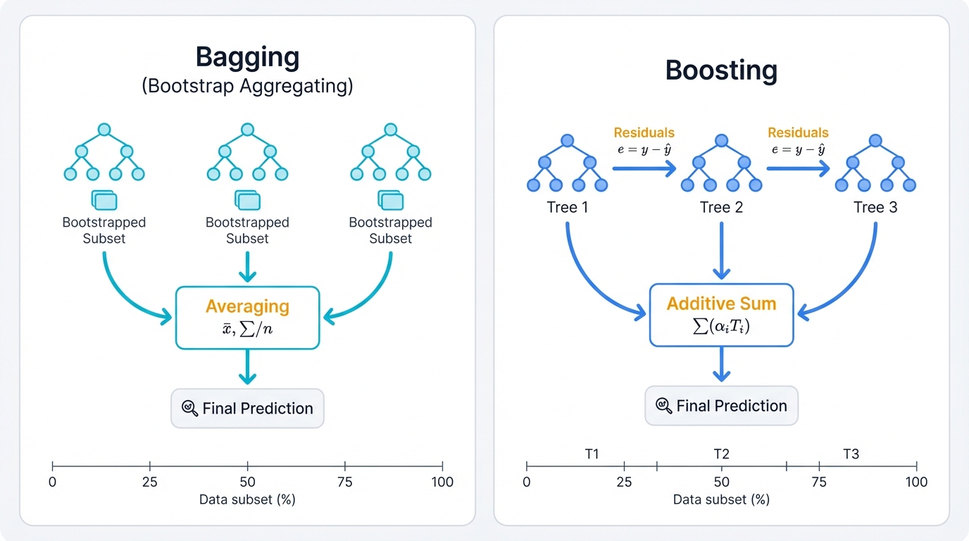
Two main ensemble strategies exist. Bagging and boosting. They solve different aspects of the bias-variance tradeoff, that fundamental tension in machine learning where models either underfit (high bias) or overfit (high variance). Bagging—Bootstrap Aggregating—reduces variance by training multiple independent models in parallel on different random data subsets, then averaging their predictions to smooth out individual errors. Random Forest exemplifies this approach: many trees trained on bootstrapped samples, combined through averaging or voting to create stable predictions. Boosting takes the opposite path, reducing bias through sequential training where each new model focuses on the errors previous models made, creating an additive ensemble where later models explicitly correct earlier mistakes through a process of iterative refinement that turns weak learners into powerful predictors.
1.2 A Brief History: The Path from AdaBoost to Gradient Boosting
Start with a question. A simple one. Can weak learners create a strong learner? Michael Kearns and Leslie Valiant posed this in the late 1980s, challenging the machine learning community to think beyond single models. Robert Schapire answered "yes" in 1990, laying the theoretical foundation that would transform the field.
AdaBoost brought these ideas to life. Yoav Freund and Robert Schapire created the first successful boosting algorithm in the mid-1990s, winning them the Gödel Prize for their theoretical contributions. AdaBoost trains weak learners one after another, increasing weights on misclassified examples so subsequent learners focus on hard cases. The final prediction? Weighted voting where more accurate learners get more influence. Simple. Elegant. Revolutionary.
Then came the insight that changed everything. Leo Breiman recognized that boosting wasn't just clever re-weighting—it was optimization, a gradient descent process in disguise where each new model followed the negative gradient of a loss function, just like neural networks descending error surfaces to find optimal weights.
Jerome Friedman formalized this breakthrough. His work between 1999 and 2001 recast boosting as numerical optimization in function space, moving beyond AdaBoost's specific exponential loss to a general framework that works with any differentiable loss function. Instead of AdaBoost's weighting scheme, Gradient Boosting Machine (GBM) uses gradient descent to minimize loss. This generalization opened new doors, extending boosting from binary classification to regression, ranking, and countless other tasks where you can define a differentiable objective.
1.3 Sequential Error Correction Framework
Watch gradient boosting work. It constructs a strong predictive model F(x) through an iterative, additive process that refines predictions step by step. Start simple. F₀(x) provides the initial model—maybe just the mean of your target variable. Then add weak models hₘ(x) sequentially, each correcting the current ensemble's deficiencies.
Here's the mechanism. Each new weak learner doesn't predict the original target variable y—that would ignore what previous models already learned. Instead, it predicts the error, the residual, of the current strong model. For regression, this means error = y - Fₘ₋₁(x), the difference between what you want and what you have.
error = y - Fm-1(x)
Working Example: Gradient Boosting Sequential Error Correction
Let's see it in action. This example demonstrates the core gradient boosting algorithm step-by-step, revealing how the model iteratively improves by focusing on residuals—those errors that previous models failed to capture.
import numpy as np
import matplotlib.pyplot as plt
from sklearn.tree import DecisionTreeRegressor
from sklearn.ensemble import GradientBoostingRegressor
from sklearn.metrics import mean_squared_error

# Generate synthetic dataset to visualize gradient boosting
np.random.seed(42)
n_samples = 100
X = np.linspace(0, 10, n_samples).reshape(-1, 1)
y = 0.5 * X.ravel() + np.sin(1.5 * X.ravel()) + np.random.normal(0, 0.3, n_samples)

print("Gradient Boosting: Sequential Error Correction Demonstration")
print("=" * 58)

# Implement a simplified gradient boosting from scratch to show the process
class SimpleGradientBoosting:
    def __init__(self, n_estimators=10, learning_rate=0.1, max_depth=3):
        self.n_estimators = n_estimators
        self.learning_rate = learning_rate
        self.max_depth = max_depth
        self.trees = []
        self.initial_prediction = None

    def fit(self, X, y):
        # Initialize with mean prediction
        self.initial_prediction = np.mean(y)

        # Current predictions start with initial value
        current_predictions = np.full(len(y), self.initial_prediction)

        print(f"Initial prediction (mean): {self.initial_prediction:.3f}")
        print(f"Initial MSE: {mean_squared_error(y, current_predictions):.3f}")

        for iteration in range(self.n_estimators):
            # Calculate residuals (pseudo-residuals for MSE loss)
            residuals = y - current_predictions

            # Train weak learner on residuals
            tree = DecisionTreeRegressor(max_depth=self.max_depth, random_state=42+iteration)
            tree.fit(X, residuals)

            # Make predictions with this tree
            tree_predictions = tree.predict(X)

            # Update ensemble with learning rate
            current_predictions += self.learning_rate * tree_predictions

            # Store the tree
            self.trees.append(tree)

            # Track progress
            mse = mean_squared_error(y, current_predictions)
            residual_std = np.std(residuals)

            print(f"Iteration {iteration+1:2d}: MSE={mse:.3f}, Residual_std={residual_std:.3f}")

            if iteration < 5:  # Show detailed info for first few iterations
                print(f"    Tree depth: {tree.get_depth()}, Tree leaves: {tree.get_n_leaves()}")
                print(f"    Residual range: [{residuals.min():.3f}, {residuals.max():.3f}]")

        return self

    def predict(self, X):
        predictions = np.full(len(X), self.initial_prediction)
        for tree in self.trees:
            predictions += self.learning_rate * tree.predict(X)
        return predictions

# Train our simple gradient boosting
print("\nTraining Simple Gradient Boosting:")
simple_gb = SimpleGradientBoosting(n_estimators=20, learning_rate=0.1, max_depth=3)
simple_gb.fit(X, y)

# Compare with sklearn's implementation
sklearn_gb = GradientBoostingRegressor(n_estimators=20, learning_rate=0.1, max_depth=3, random_state=42)
sklearn_gb.fit(X, y)

# Make predictions
X_test = np.linspace(0, 10, 200).reshape(-1, 1)
simple_predictions = simple_gb.predict(X_test)
sklearn_predictions = sklearn_gb.predict(X_test)

print(f"\nFinal comparison:")
print(f"Simple GB final MSE: {mean_squared_error(y, simple_gb.predict(X)):.3f}")
print(f"Sklearn GB final MSE: {mean_squared_error(y, sklearn_gb.predict(X)):.3f}")

# Demonstrate the additive nature of gradient boosting
print(f"\nAdditive Model Demonstration:")
print("-" * 29)

# Show how predictions build up over iterations
cumulative_predictions = np.full((len(X_test), len(simple_gb.trees) + 1), simple_gb.initial_prediction)

for i, tree in enumerate(simple_gb.trees):
    tree_contrib = simple_gb.learning_rate * tree.predict(X_test)
    cumulative_predictions[:, i+1] = cumulative_predictions[:, i] + tree_contrib

    if i < 5:  # Show first few trees
        print(f"After tree {i+1}: Contribution range [{tree_contrib.min():.3f}, {tree_contrib.max():.3f}]")

# Visualization of the boosting process
fig, axes = plt.subplots(2, 3, figsize=(18, 12))

# Plot 1: Original data and final prediction
axes[0, 0].scatter(X, y, alpha=0.6, s=20, label='Data')
axes[0, 0].plot(X_test, simple_predictions, 'r-', label='Simple GB', linewidth=2)
axes[0, 0].plot(X_test, sklearn_predictions, 'g--', label='Sklearn GB', linewidth=2)
axes[0, 0].set_title('Final Predictions')
axes[0, 0].set_xlabel('X')
axes[0, 0].set_ylabel('y')
axes[0, 0].legend()

# Plot 2: Convergence of MSE
train_errors = []
current_pred = np.full(len(X), simple_gb.initial_prediction)
train_errors.append(mean_squared_error(y, current_pred))

for tree in simple_gb.trees:
    current_pred += simple_gb.learning_rate * tree.predict(X)
    train_errors.append(mean_squared_error(y, current_pred))

axes[0, 1].plot(range(len(train_errors)), train_errors, 'b-o', markersize=4)
axes[0, 1].set_title('Training Error Convergence')
axes[0, 1].set_xlabel('Iteration')
axes[0, 1].set_ylabel('MSE')
axes[0, 1].grid(True, alpha=0.3)

# Plot 3: Individual tree contributions
iterations_to_show = [0, 1, 4, 9, 19]
for i, iter_num in enumerate(iterations_to_show):
    if iter_num < len(simple_gb.trees):
        tree_pred = simple_gb.learning_rate * simple_gb.trees[iter_num].predict(X_test)
        axes[0, 2].plot(X_test, tree_pred, alpha=0.7, label=f'Tree {iter_num+1}')

axes[0, 2].set_title('Individual Tree Contributions')
axes[0, 2].set_xlabel('X')
axes[0, 2].set_ylabel('Tree Prediction')
axes[0, 2].legend()

# Plot 4: Cumulative predictions over iterations
iterations_to_plot = [0, 2, 5, 10, 20]
for iter_num in iterations_to_plot:
    if iter_num < cumulative_predictions.shape[1]:
        axes[1, 0].plot(X_test, cumulative_predictions[:, iter_num],
                       alpha=0.7, label=f'After {iter_num} trees')

axes[1, 0].scatter(X, y, alpha=0.4, s=15, color='black')
axes[1, 0].set_title('Cumulative Predictions Build-up')
axes[1, 0].set_xlabel('X')
axes[1, 0].set_ylabel('Prediction')
axes[1, 0].legend()

# Plot 5: Residuals evolution
residuals_over_time = []
current_pred = np.full(len(X), simple_gb.initial_prediction)
residuals_over_time.append(y - current_pred)

for tree in simple_gb.trees[:10]:  # First 10 trees
    current_pred += simple_gb.learning_rate * tree.predict(X)
    residuals_over_time.append(y - current_pred)

residual_stds = [np.std(residuals) for residuals in residuals_over_time]
axes[1, 1].plot(range(len(residual_stds)), residual_stds, 'r-o', markersize=4)
axes[1, 1].set_title('Residual Standard Deviation')
axes[1, 1].set_xlabel('Iteration')
axes[1, 1].set_ylabel('Std(Residuals)')
axes[1, 1].grid(True, alpha=0.3)

# Plot 6: Feature importance (tree depth analysis)
tree_depths = [tree.get_depth() for tree in simple_gb.trees]
tree_leaves = [tree.get_n_leaves() for tree in simple_gb.trees]

axes[1, 2].plot(range(1, len(tree_depths)+1), tree_depths, 'g-o', markersize=4, label='Tree Depth')
ax2 = axes[1, 2].twinx()
ax2.plot(range(1, len(tree_leaves)+1), tree_leaves, 'orange', marker='s', markersize=4, label='Leaves')
axes[1, 2].set_xlabel('Tree Number')
axes[1, 2].set_ylabel('Tree Depth', color='g')
ax2.set_ylabel('Number of Leaves', color='orange')
axes[1, 2].set_title('Tree Complexity Over Iterations')
axes[1, 2].legend(loc='upper left')
ax2.legend(loc='upper right')

plt.tight_layout()
plt.savefig('gradient_boosting_process.png', dpi=150, bbox_inches='tight')
print(f"\nGradient boosting process visualization saved as 'gradient_boosting_process.png'")

# Key insights about the additive process
print(f"\nKey Insights about Sequential Error Correction:")
print("- Each tree learns from residuals of the current ensemble")
print("- Learning rate controls how much each tree contributes")
print("- Residuals get smaller over iterations (if not overfitting)")
print("- Final prediction = initial_pred + sum(learning_rate * tree_predictions)")
print(f"- Additive nature: F_m(x) = F_0(x) + Σ(η * h_m(x))")
Watch what this implementation reveals. Sequential error correction through additive modeling—that's gradient boosting's core mechanism, distilled to its essence. Each tree learns to predict the residuals, those errors that previous models couldn't capture. The ensemble gradually refines its predictions, getting closer to the true target with each iteration. The learning rate? It controls how aggressively each tree's contribution gets incorporated, balancing between rapid convergence and careful refinement that prevents overfitting while enabling optimal solutions.
Section 2: The Gradient Boosting Machine (GBM) Algorithm
2.1 Functional Optimization: Gradient Descent on Loss Functions
Fitting residuals sequentially works. But it's just one instance of something bigger. Much bigger. GBM formalizes this as gradient descent optimization in function space—a conceptual leap that transforms boosting from a specific algorithm into a general framework where the parameters being optimized aren't numerical weights but entire functions, the weak learners themselves.
The objective? Find function F(x) that minimizes your chosen loss function L(y, F(x)). This loss quantifies the gap between true targets y and model predictions F(x). Your choice of loss function determines everything about how your model learns. Regression problems use Mean Squared Error (MSE), L(y, F) = ½(y - F)², which penalizes prediction errors quadratically, making large errors hurt more than small ones. Classification tasks employ Log-Loss (Cross-Entropy), L(y, F) = y log(p) + (1-y) log(1-p), which measures how well predicted probabilities match actual class labels, heavily penalizing confident wrong predictions.
The key GBM insight? Adding a new weak learner hm(x) to existing ensemble Fm-1(x) is analogous to taking a gradient descent step in parameter space. The algorithm adds a function pointing in the negative gradient direction of the loss function—the direction of steepest descent in the loss landscape, the path that most effectively reduces overall error with each step.
2.2. The Role of Pseudo-Residuals
Functional gradient descent sounds abstract. Pseudo-residuals make it practical. For each training instance i at iteration m, the pseudo-residual rim is the negative gradient of the loss function evaluated at the previous model's prediction Fm-1(xi).
$$r_{im} = -\left[\frac{\partial L(y_i, F(x_i))}{\partial F(x_i)}\right]_{F(x_i)=F_{m-1}(x_i)}$$
This formulation's power lies in its generality. For MSE loss, L(y, F) = ½(y - F)², the partial derivative is -(y - F). The negative of this? Simply (y - F), the standard residual. Thus, for regression with MSE, fitting pseudo-residuals is identical to fitting errors—the intuitive approach we started with. But use different loss functions and the same algorithm applies to countless problems. For Log-Loss in classification, the pseudo-residuals become (y - p), where p is the predicted probability, driving the model to correct its probability estimates through iterative refinement that focuses computational effort where predictions need the most improvement.
This generalization represents a conceptual leap. It moves beyond AdaBoost's specific exponential loss function and re-weighting scheme, revealing AdaBoost as just one instance within the broader GBM family. This abstraction enables modern GBDTs to tackle not only classification and regression but also complex tasks like learning-to-rank (using loss functions like LambdaMART) or even custom business objectives, provided they can be expressed as differentiable loss functions that guide the gradient descent process.
2.3. The Iterative Process: A Step-by-Step Walkthrough
The generic GBM algorithm follows a systematic sequence:
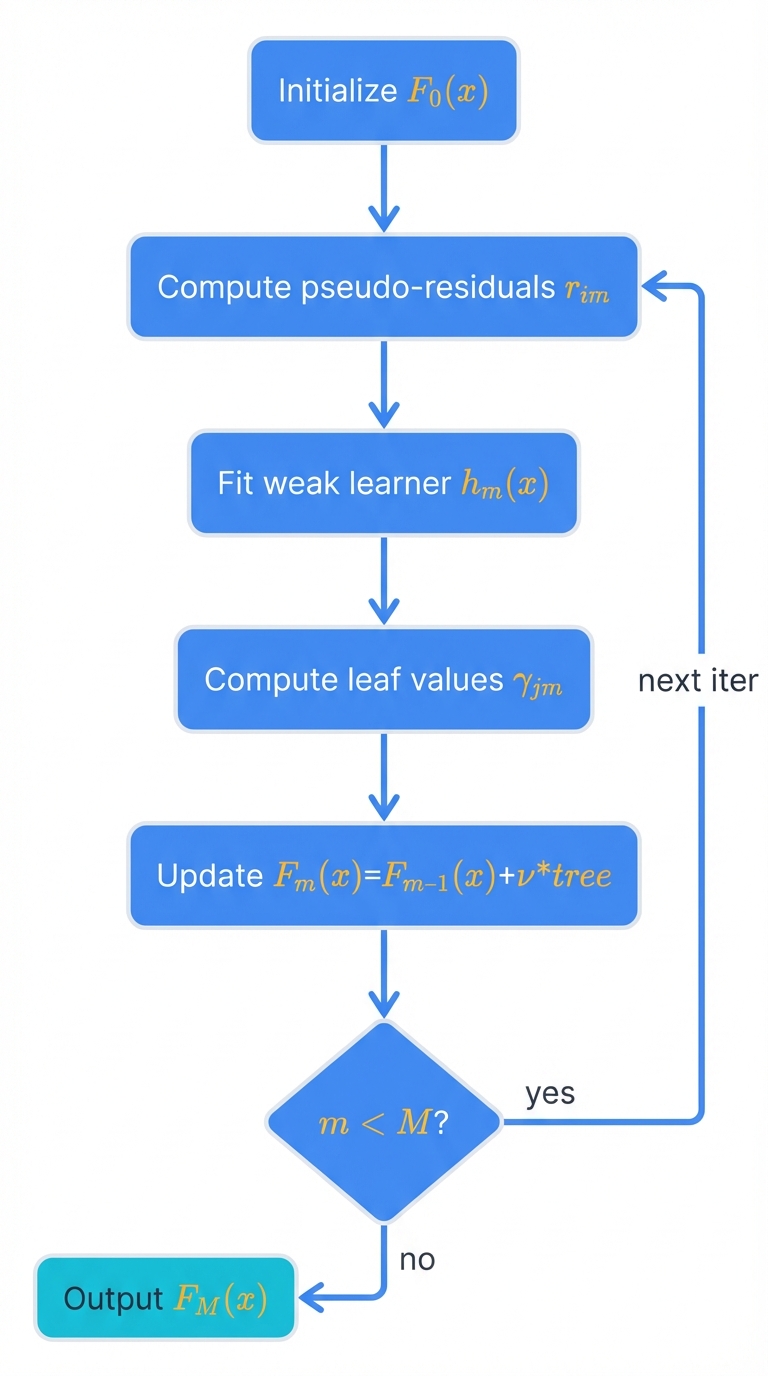
Initialization. Create an initial, simple model F₀(x). This constant value minimizes the loss function over the entire dataset. For MSE in regression? The mean of target variable y. For Log-Loss in classification? The log-odds of the positive class. Simple. Effective.
$$F_0(x) = \arg\min_{\gamma} \sum_{i=1}^N L(y_i, \gamma)$$
Iteration m = 1 to M. For each of M boosting rounds:
a. Compute Pseudo-Residuals. For each training sample i=1,..., N, calculate pseudo-residual rim as the negative gradient of the loss function with respect to previous iteration's prediction Fm-1(xi).
b. Fit a Weak Learner. Train a weak learner, typically a regression decision tree hm(x), using features X as input and calculated pseudo-residuals {r1m,..., rNm} as target labels. The tree partitions data into regions that best predict these pseudo-residuals.
c. Compute Optimal Leaf Values. For each terminal leaf region Rjm of new tree hm(x), determine optimal output value γjm. This value minimizes the loss function for all samples falling into that leaf.
$$\gamma_{jm} = \arg\min_{\gamma} \sum_{x_i \in R_{jm}} L(y_i, F_{m-1}(x_i) + \gamma)$$
Friedman's "TreeBoost" algorithm proposed this step. Finding separate optimal values for each leaf? More refined than finding a single multiplier for the whole tree.
d. Update the Model. Update the full ensemble model by adding the new weak learner, scaled by learning rate ν.
$$F_m(x) = F_{m-1}(x) + \nu \sum_{j=1}^{J_m} \gamma_{jm} I(x \in R_{jm})$$
where I is the indicator function.
Output. The final model FM(x) is the sum of the initial model and all sequentially trained weak learners.
Visual Description. Imagine this iterative process as a function approximation machine. The initial flat line of F₀(x) provides the first guess. The first tree h₁(x) adds a few step-like corrections, creating F₁(x). The second tree h₂(x) adds smaller, more refined steps to correct remaining errors, creating F₂(x). Each iteration adds another layer of detail, allowing the final function FM(x) to trace complex patterns in the data with high fidelity, capturing relationships that would be impossible for any single model to represent accurately.
2.4. Key Control Mechanisms: Learning Rate (Shrinkage) and Early Stopping
Two hyperparameters control GBM behavior more than any others. Learning rate and number of iterations, managed via early stopping.
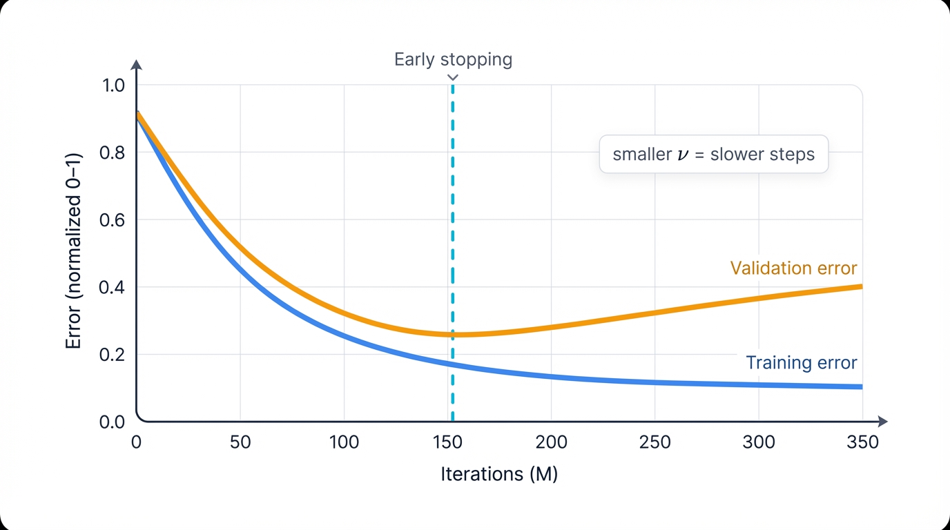
Learning Rate (ν) / Shrinkage. This parameter scales each new tree's contribution before adding it to the ensemble. Small values between 0.01 and 0.3 work best. Why? It prevents overfitting. A smaller learning rate forces the model to take smaller, more cautious steps in optimization. This requires more iterations (M) to achieve the same training error, but the resulting model generalizes much better to unseen data—a pattern directly analogous to learning rates in deep learning optimization algorithms like stochastic gradient descent.
Shrinkage does more than slow learning. It alters the solution path itself. Without shrinkage (ν=1), the model aggressively fits full pseudo-residuals at each step, learning noise and training set artifacts. Smaller steps compel the model to build a more diverse ensemble where no single tree dominates predictions. Each contributes only a small correction, forcing the algorithm to identify patterns that consistently appear across many small adjustments—patterns far more likely to represent generalizable signals rather than random noise. This functions as powerful implicit regularization, explaining why combining low learning rates with high estimator counts is a near-universal best practice for GBDTs.
Number of Iterations (M) / n_estimators. This determines total weak learners in the final model. A direct tradeoff exists: more trees increase model complexity and decrease training error. But beyond a certain point? Overfitting begins, degrading performance on unseen data.
Early Stopping. Finding optimal M manually is impractical. Use early stopping instead. Monitor model performance on a separate validation dataset during training. Halt the training process when validation performance stops improving for a specified number of consecutive iterations. This technique automatically finds an effective M, preventing the model from continuing to train once it has started to overfit—a simple but powerful regularization method that saves computational resources while improving generalization.
Part II: Technical Deep Dive into Modern Implementations
Theory provides foundation. Implementation delivers results. This part transitions from foundational GBM to detailed examination of three leading modern libraries: XGBoost, LightGBM, and CatBoost. Each section dissects specific algorithmic innovations and system-level optimizations that differentiate these frameworks from the original GBM and from one another, establishing their respective strengths and design philosophies.
Section 3: XGBoost (eXtreme Gradient Boosting)
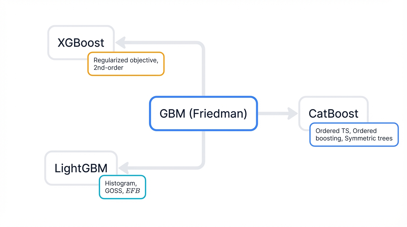
XGBoost changed everything. Tianqi Chen and Carlos Guestrin's open-source library rose to prominence through consistent success in machine learning competitions and is renowned for performance, feature richness, and efficiency. Its primary innovations? A regularized learning objective, more accurate optimization, and sophisticated system design for scalability.
3.1. Algorithmic Enhancements: Regularized Objective Function and Second-Order Approximation
The core mathematical innovation of XGBoost is its carefully formulated objective function. Explicit regularization controls model complexity. Prevents overfitting.
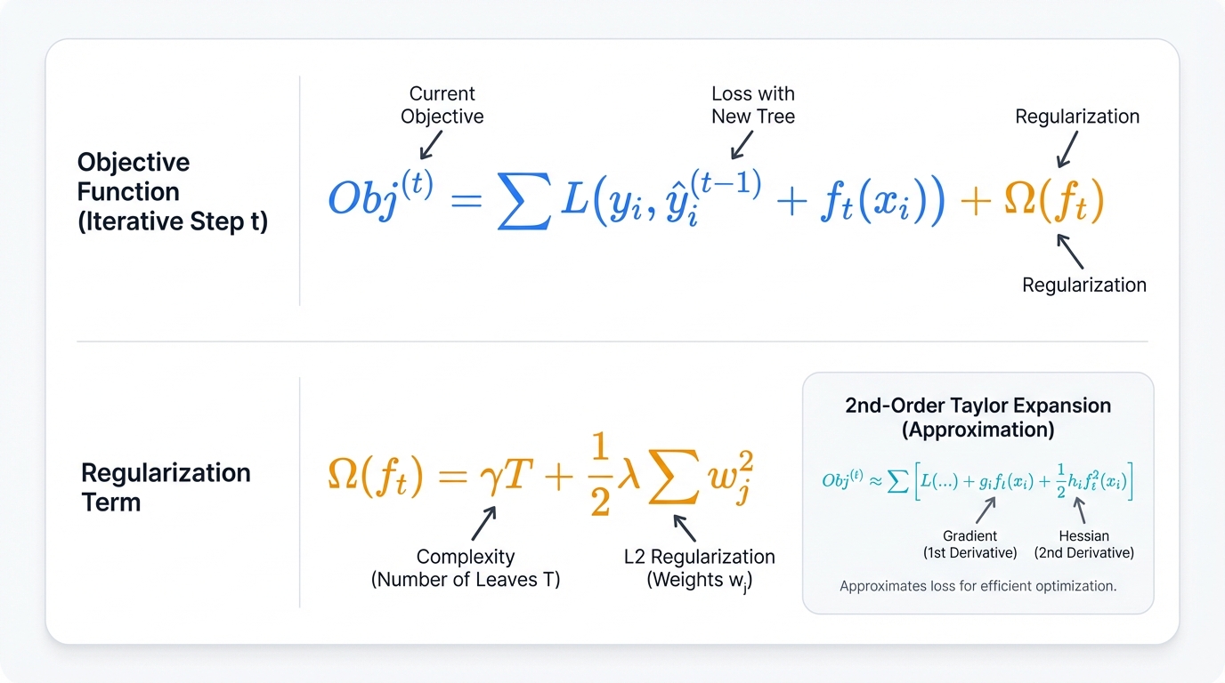
Regularized Objective Function. Unlike standard GBM, which only seeks to minimize loss, XGBoost's objective at each step includes a penalty term for the complexity of the new tree being added. The objective function at iteration t:
$$\text{Obj}^{(t)} = \sum_{i=1}^n L(y_i, \hat{y}_i^{(t-1)} + f_t(x_i)) + \Omega(f_t)$$
Here, L is the loss function, $\hat{y}_i^{(t-1)}$ is the prediction from previous t-1 trees, and ft is the new tree. The regularization term, Ω(ft), penalizes the complexity of this new tree:
$$\Omega(f_t) = \gamma T + \frac{1}{2}\lambda \sum_{j=1}^T w_j^2$$
Second-Order Approximation. To efficiently optimize this regularized objective, XGBoost employs a second-order Taylor expansion of the loss function around the current prediction—a significant departure from traditional GBM, which uses only the first derivative (the gradient). The Taylor expansion approximates the objective as:
$$\text{Obj}^{(t)} \approx \sum_{i=1}^n \left[L(y_i, \hat{y}_i^{(t-1)}) + g_i f_t(x_i) + \frac{1}{2}h_i f_t^2(x_i)\right] + \Omega(f_t)$$
where gi and hi are first and second-order derivatives (gradient and Hessian) of the loss function with respect to prediction $\hat{y}_i^{(t-1)}$. This quadratic approximation provides a more accurate picture of the loss function's landscape, allowing the algorithm to take more direct and effective steps towards the minimum, resulting in faster convergence.
3.2. System Optimizations: Sparsity-Aware Split Finding and Parallelization
Beyond algorithmic improvements, XGBoost's success comes from thoughtful system design. Optimizations for modern hardware. Real-world data challenges.
Sparsity-Aware Split Finding. One of the most impactful features detailed in the original XGBoost paper? A novel algorithm for handling sparse data and missing values efficiently. Instead of requiring users to impute missing values beforehand, XGBoost learns how to handle them during training. When evaluating a potential split on a feature, the algorithm considers two scenarios: sending instances with missing values to the left child node, or sending them to the right. It calculates gain for both scenarios and learns a "default direction" for missing values at each node—the direction that maximizes gain. This allows the model to learn the predictive meaning of missingness directly from data, which proves more effective than naive imputation.
Parallelization and Cache-Awareness. While the boosting process of adding trees is inherently sequential, individual tree construction offers opportunities for parallelization. XGBoost parallelizes the most computationally intensive part of tree building: the search for the best split. Data gets sorted by feature values, and the process of scanning through these values to find the best split point is parallelized across CPU threads. Furthermore, XGBoost is designed with hardware in mind through cache-aware algorithms that organize data in memory to minimize cache misses and out-of-core computation that processes datasets too large to fit into RAM by splitting data into blocks and storing them on disk.
3.3. Visualizing the XGBoost Tree-Building Process
The construction of a single tree in XGBoost follows a systematic process driven by the regularized objective function.
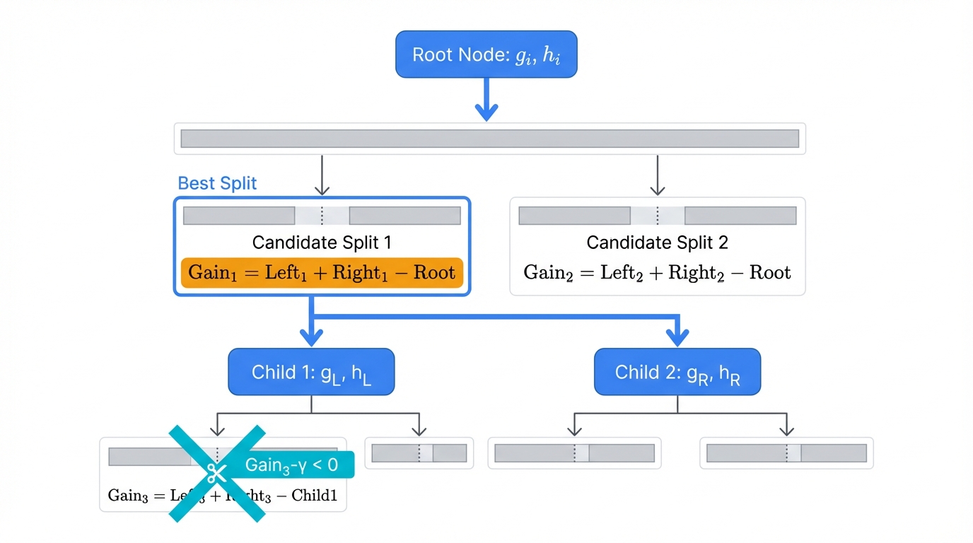
Visual Description of the Process:
Initialization. Begin with all training instances (represented by their gradients gi and Hessians hi) in the root node.
Similarity Score Calculation. For any given set of instances in a node, XGBoost calculates a Similarity Score derived from the objective function that measures node purity:
$$\text{Similarity Score} = \frac{(\sum g_i)^2}{\sum h_i + \lambda}$$
Gain Calculation for Splits. The algorithm iterates through every feature and every possible split point for that feature. For each potential split, it partitions instances into left and right child nodes and calculates Gain:
$$\text{Gain} = \text{Similarity}_{\text{Left}} + \text{Similarity}_{\text{Right}} - \text{Similarity}_{\text{Root}}$$
Best Split Selection. The split yielding highest gain across all features and all values gets selected as the best split for the current node.
Recursive Growth. This process repeats for newly created child nodes, continuing until a stopping criterion like reaching max_depth is met.
Pruning. After a tree is fully grown to its max_depth, XGBoost performs post-pruning. It traverses the tree from bottom up. For each split, it evaluates if gain from that split is less than the regularization parameter γ. If Gain - γ < 0, the split is considered not worthwhile, and the branch gets pruned (removed). This pruning strategy proves more robust than pre-pruning (early stopping) used in standard GBM, as it can remove splits that looked promising initially but proved ineffective after further splits were made deeper in the tree.
Several Python libraries, including matplotlib (via xgboost.plot_tree), graphviz, and the more advanced dtreeviz, generate visual representations of final tree structures, aiding model interpretation.
Section 4: LightGBM (Light Gradient Boosting Machine)
Speed. Efficiency. Scale. Microsoft built LightGBM with a singular focus on these priorities, particularly for large datasets. It introduces novel techniques that fundamentally alter the tree-building process to reduce computational complexity and memory usage without significant compromises in accuracy.
4.1. The Pursuit of Speed: Histogram-Based Algorithms
The most significant source of LightGBM's speed advantage? Histogram-based algorithms for finding the best splits in decision trees. Traditional GBDT implementations, including the exact method in XGBoost, use a pre-sorted algorithm that sorts values for every continuous feature for every node—an operation with time complexity O(#data × log(#data)).
LightGBM avoids this expensive step. First, it discretizes continuous feature values into a fixed number of bins (e.g., 255). Then it constructs a histogram for each feature based on these bins. Finding the best split point reduces to iterating through discrete bins of the histogram (O(#bins)) rather than individual data points (O(#data)). Since the number of bins is typically much smaller than the number of data points, this approach is dramatically faster. Furthermore, this method significantly reduces memory usage—the algorithm only needs to store discrete bin values instead of original continuous feature values.
4.2. Intelligent Sampling: Gradient-based One-Side Sampling (GOSS)
To further accelerate training on large datasets, LightGBM introduces Gradient-based One-Side Sampling (GOSS). The intuition? Not all data instances contribute equally to training. Instances for which the model already makes accurate predictions have small gradients. Instances that are poorly predicted (under-trained) have large gradients. These large-gradient instances are more informative for finding optimal splits.
GOSS leverages this insight through non-uniform sampling:
Keep all instances with large gradients (the "hard" examples).
Perform random sampling on remaining instances with small gradients (the "easy" examples).
Amplify the contribution of sampled small-gradient instances by a constant factor when calculating information gain to maintain data distribution integrity.
This method allows LightGBM to focus computational efforts on the most informative data points, achieving a good approximation of true information gain with a much smaller dataset, thereby speeding up training significantly.
4.3. Efficient Feature Handling: Exclusive Feature Bundling (EFB)
For datasets with very high numbers of features (high dimensionality), especially sparse ones, histogram construction costs can still be substantial. Exclusive Feature Bundling (EFB) addresses this challenge based on the observation that in many sparse datasets (e.g., those with one-hot encoded features), many features are mutually exclusive—they rarely take non-zero values simultaneously.
EFB identifies such features and bundles them into single, denser features. This is done by creating offsets in bin ranges, allowing multiple features to coexist in the same bundled feature without collision. By reducing the effective number of features, EFB significantly lowers histogram construction complexity from O(#data × #feature) to O(#data × #bundle), where #bundle ≪ #feature. The original paper proves that finding optimal bundling is NP-hard (reducible to graph coloring) but demonstrates that a greedy algorithm provides an effective approximation in practice.
4.4. A Different Growth Strategy: Understanding Leaf-Wise Tree Growth
LightGBM's default tree growth strategy is another key differentiator that impacts both performance and model structure.
Visual and Conceptual Comparison of Growth Strategies:
Level-wise (or Depth-wise) Growth. This is the traditional approach used by most GBDT implementations, including XGBoost. The tree is built symmetrically, level by level. All nodes at a given depth are split before the algorithm proceeds to the next deeper level. This results in balanced trees and is less prone to overfitting on smaller datasets, as it acts as implicit regularization.
Leaf-wise (or Best-first) Growth. This is LightGBM's strategy. Instead of expanding all nodes at a given level, the algorithm identifies the single leaf node anywhere in the tree that will yield the largest reduction in loss (the highest gain) and splits it. This process repeats, leading to growth of an asymmetric tree where some branches become much deeper than others. This "greedy" approach allows the model to converge to lower loss more quickly than level-wise strategy, as it focuses computational effort where it's most effective. However, this same greediness makes it more susceptible to overfitting on smaller datasets—behavior that must be controlled with regularization parameters like num_leaves and max_depth.
Section 5: CatBoost (Categorical Boosting)
Yandex built CatBoost to solve problems that academic papers ignored but production systems encountered daily. Real datasets contain categorical features. User IDs. Product codes. Geographic regions. Traditional gradient boosting handles them poorly. Worse, subtle target leakage in standard implementations biases models and inflates validation scores.
CatBoost addresses both issues through statistical rigor. Its name combines "Categorical" and "Boosting," reflecting its core mission: handle categorical features correctly while eliminating prediction shift bias.
5.1 Solving the Categorical Challenge: Ordered Target Statistics
Important Consideration: While this approach offers significant benefits, it's crucial to understand its limitations and potential challenges as outlined in this section.
CatBoost's primary innovation solves categorical feature handling through statistical rigor. Other libraries force awkward preprocessing. One-hot encoding explodes feature dimensions (1000 categories = 1000 features). Label encoding imposes false ordinal relationships (encoding cities as 1, 2, 3 implies Chicago > Boston > Austin). CatBoost handles categories natively. Correctly.
A common technique for high-cardinality categorical features is target encoding (mean encoding). Replace each category with the average target value for that category. Seems clever: encode "Ford" as the average car price for Ford vehicles.
But naive target encoding creates target leakage. When calculating the encoding for a Ford Mustang priced at $35,000, you include that same $35,000 in the average. The feature value depends partly on the target you're trying to predict—a circular dependency that inflates model performance and causes severe overfitting.
Ordered Target Statistics (Ordered TS) solves this through temporal simulation. CatBoost randomly permutes the data, then calculates target statistics using only instances that appear before the current instance in this permutation, ensuring the encoding for each instance uses independent information and prevents leakage. Multiple random permutations during training make this process robust.
5.2 Preventing Target Leakage: The Ordered Boosting Algorithm
CatBoost extends the ordering principle beyond feature encoding to the core boosting process. This combats "prediction shift"—a subtle bias where gradients calculated on training data differ from gradients you'd see on test data. Standard gradient boosting unknowingly creates this bias.
Ordered Boosting addresses this by separating tree structure decisions from residual calculations. Standard GBDT uses the same data points to build tree structure and calculate residuals for the next tree—creating subtle dependencies.
Ordered Boosting calculates residuals for sample k using a model trained on only the first k-1 samples of a random permutation, ensuring gradient estimates are unbiased with respect to the model that generated them. The result? More robust models that generalize better to unseen data.
5.3 Architectural Uniqueness: Symmetric (Oblivious) Trees
CatBoost takes a radically different approach to tree architecture. While XGBoost uses level-wise growth and LightGBM uses leaf-wise growth, CatBoost builds symmetric (oblivious) trees with a unique constraint.
Visual and Conceptual Description of Symmetric Trees:
CatBoost builds symmetric (oblivious) decision trees where all nodes at the same depth use identical splitting rules. If depth 0 splits on "age > 30", every node at depth 0 applies this same rule. If depth 1 splits on "income < $50k", every node at depth 1 uses this condition.
This creates perfectly balanced trees with severe complexity constraints. The structure acts as powerful implicit regularization, preventing trees from fitting training noise. The practical benefit? Extremely fast inference. Instead of following sequential if-then-else chains, predictions use vectorized operations that execute in parallel across tree levels.
These three libraries embody distinct philosophies that reveal fundamental trade-offs in model engineering:
XGBoost. Robustness through algorithmic rigor and system co-design. Enhances core boosting mathematics while building efficient execution systems.
LightGBM. Raw speed through clever approximation. Fundamentally alters data processing via histograms and sampling to make computation cheaper.
CatBoost. Statistical integrity and reliability. Solves deep-seated issues like target leakage through novel permutation-based techniques.
Choosing a library isn't just about performance. It's a strategic decision based on your primary constraints: computational resources, data characteristics, or statistical guarantee requirements.
The distinct tree growth strategies function as implicit regularization mechanisms. Level-wise growth (XGBoost) builds trees breadth-first, creating inherently constrained structures that prevent rapid over-specialization by ensuring balanced development across all branches. Leaf-wise growth (LightGBM) takes a greedy and flexible approach, expanding the most beneficial leaf at each step to find complex patterns faster, though this risks overfitting in small datasets. Symmetric growth (CatBoost) imposes the most restrictive approach, using strong structural constraints that enhance overfitting resistance by ensuring perfectly balanced binary trees.
Part III: Comparative Analysis and Performance
Theory means nothing without practical guidance. This section provides evidence-based comparisons of XGBoost, LightGBM, and CatBoost across dimensions that matter: training speed, memory usage, predictive accuracy, and data type handling. You'll learn when to choose each framework based on your specific constraints and requirements.
Section 6: A Head-to-Head Comparison
6.1 Speed and Memory Efficiency: Benchmarking Training and Prediction Times
Computational performance determines whether your model trains in minutes or hours. Fits in memory or crashes your server. These differences matter enormously in production environments and during iterative experimentation.
Training Speed. LightGBM consistently wins training speed benchmarks. Its histogram-based algorithm eliminates expensive data sorting. GOSS and EFB reduce data and features processed per iteration. The result? 5-10x speedups on large datasets compared to traditional methods.
XGBoost's training speed depends heavily on the tree_method parameter. The original "exact" method is slow. The "hist" method (now default) implements histogram-based splitting similar to LightGBM, closing the performance gap significantly.
CatBoost trains slower on CPU due to computational overhead from permutation-based strategies (Ordered TS and Ordered Boosting). Statistical robustness requires more computation—a classic accuracy-speed tradeoff.
Prediction (Inference) Speed. CatBoost excels at inference despite slower training. Symmetric tree structure enables vectorized prediction calculations that often outperform XGBoost and LightGBM in low-latency production environments, making CatBoost attractive for high-throughput serving.
Memory Usage. LightGBM wins memory efficiency through histogram-based integer binning. Storing 255 bins per feature uses far less memory than storing millions of continuous values. This advantage becomes critical with datasets approaching memory limits.
6.2 Predictive Accuracy on Standard Datasets
Speed matters. Accuracy wins. All three libraries achieve exceptional performance on tabular data—they routinely dominate Kaggle leaderboards and power production systems at major tech companies.
No single library universally dominates. The "best" choice depends on your dataset's characteristics and your specific requirements.
CatBoost excels on datasets with many meaningful categorical features. Ordered Target Statistics provides statistically sound encoding without target leakage, extracting more signal than manual preprocessing approaches. E-commerce, marketing, and recommendation datasets particularly benefit.
XGBoost functions as the reliable all-rounder. Its regularized objective, second-order optimization, and extensive hyperparameter options provide robust performance across diverse problem types. XGBoost's Kaggle dominance from 2014-2018 established its reputation as the "safe choice."
LightGBM matches XGBoost's accuracy while training much faster. Its aggressive leaf-wise growth finds optimal solutions quickly but requires careful tuning on smaller datasets. The num_leaves parameter becomes critical for controlling overfitting—set it too high and the model memorizes noise.
Benchmarking datasets include UCI Machine Learning Repository standards (Higgs, Epsilon, Covertype) and Kaggle competitions (Titanic, Santander Customer Transaction Prediction, House Prices). These provide consistent baselines for performance comparison.
6.3 Handling of Categorical and Missing Data: A Key Differentiator
Real datasets are messy. They contain categorical features that resist numerical encoding. Missing values that break naive algorithms. How each library handles these imperfections determines practical usability more than raw performance metrics.
Categorical Data:
CatBoost. Categorical handling is CatBoost's signature strength. Simply specify categorical column indices. The library handles encoding internally using Ordered Target Statistics. No preprocessing required. No target leakage. No feature explosion from one-hot encoding.
LightGBM. Provides native categorical support through specialized algorithms that partition categories into optimal subsets. More sophisticated than manual encoding. Less statistically rigorous than CatBoost's approach. Requires casting columns to pandas 'category' dtype.
XGBoost. Historically required manual preprocessing (one-hot or label encoding). Recent versions added experimental categorical support with enable_categorical=True, but this functionality remains less mature than LightGBM or CatBoost.
Missing Data:
All three libraries handle missing values (NaN) natively. Mandatory imputation? Eliminated.
XGBoost. Uses sparsity-aware split finding. At each node, it learns a "default direction" for missing values—left or right child—based on which assignment maximizes information gain.
LightGBM. Treats missing values as a distinct group. During training, it learns whether sending missing values left or right optimizes split gain for each node.
CatBoost. Handles missing values automatically. For numerical features, it learns optimal split directions. For categorical features, missing values become an additional category. The nan_mode parameter allows explicit control over missing value treatment.
Table 1: Comparative Overview of XGBoost, LightGBM, and CatBoost
| Feature | XGBoost | LightGBM | CatBoost |
|---|---|---|---|
| Primary Innovation | Regularized objective, second-order optimization, system scalability | Histogram-based splits, GOSS, EFB for speed and efficiency | Ordered Boosting and Ordered Target Statistics for categorical data |
| Tree Growth | Level-wise (default), configurable to leaf-wise | Leaf-wise (best-first), optimized for faster convergence | Symmetric (Oblivious), highly regularized |
| Categorical Features | Manual preprocessing required; experimental native support | Native support via equality splits; requires 'category' dtype | Native support, handles automatically, no preprocessing |
| Missing Values | Native handling via default direction learning | Native handling via optimal direction learning | Native handling; separate category or default direction |
| Training Speed | Fast (with hist method), typically slower than LightGBM | Very fast; generally fastest, especially on large datasets | Slower due to permutation overhead |
| Inference Speed | Fast | Fast | Very fast due to vectorized symmetric trees |
| Memory Usage | Moderate to high (exact method) | Low; histogram binning efficiency | Moderate |
| Regularization | Strong; explicit L1/L2 + gamma pruning | Strong; L1/L2 + tree complexity controls | Strong; L2 + implicit from ordered boosting |
| Ideal Use Case | Robust all-rounder; strong community support | Large datasets requiring speed and memory efficiency | Datasets with many categorical features; overfitting resistance |
Section 7: Computational Requirements and Scalability
Modern gradient boosting libraries must handle datasets that exceed single-machine memory. Leverage contemporary hardware architectures. Scalability determines whether you can solve real-world problems or remain constrained to toy datasets.
7.1 CPU vs. GPU Performance
GPU acceleration transforms training times. Hours become minutes on large datasets. 10x+ speedups are common. All three libraries provide mature GPU implementations, but performance characteristics differ.
CPU Performance. XGBoost historically held slight advantages on CPU through optimized system design and mature codebase. LightGBM's histogram algorithms also perform excellently on CPU architectures.
GPU Performance. LightGBM often excels on GPU due to algorithms designed for parallel architectures. CatBoost's symmetric tree structure maps naturally to GPU parallelism, providing efficient training and inference.
Choose GPU when dataset size exceeds 100k+ rows or training time becomes a bottleneck. The speedup justifies the additional complexity.
7.2 Behavior with Large-Scale Datasets
Modern GBDT libraries overcome scalability limitations that plagued earlier implementations. They handle datasets that would crash traditional algorithms.
LightGBM dominates extremely large datasets. Millions to billions of rows. Its histogram algorithms, GOSS sampling, and EFB feature bundling create unmatched memory efficiency and training speed. Choose LightGBM when memory or time constraints are primary concerns.
XGBoost provides robust scalability through out-of-core computation. It trains on datasets larger than RAM by intelligently managing data blocks between disk and memory, making XGBoost reliable for enterprise-scale problems where stability matters more than raw speed.
CatBoost scales effectively to large datasets, with particularly efficient GPU implementations. Its permutation-based algorithms add computational overhead but remain practical for most real-world sizes.
7.3 Integration with Distributed Computing Frameworks
Truly massive datasets require distributed computing. Machine clusters. All three libraries integrate with major distributed frameworks, enabling horizontal scaling beyond single-machine limits.
Dask Integration. All libraries work with Dask for distributed Python computing, scaling across clusters while maintaining familiar APIs.
Apache Spark Integration. Enterprise environments use Spark for big data pipelines. XGBoost has the most mature Spark integration, with years of production deployment. LightGBM and CatBoost provide newer but functional Spark support.
XGBoost leads in distributed ecosystem maturity. Its long deployment history on Hadoop and Spark platforms provides confidence for enterprise adoption. Extensive documentation and community support reduce integration risks.
This analysis confirms the "No Free Lunch" theorem. No single GBDT library dominates universally. Optimal choice depends on dataset characteristics and project constraints. For high-cardinality categorical features, choose CatBoost for its statistical rigor in handling complex categorical variables without manual encoding. For extremely large, sparse datasets, choose LightGBM for its superior speed and memory efficiency that scales to massive data volumes. For robust all-purpose applications, choose XGBoost for its proven reliability across diverse problem types and established production track record.
Feature convergence is evident across libraries. LightGBM's histogram success prompted XGBoost's "hist" method (now default). Native categorical handling success in LightGBM and CatBoost spurred XGBoost's experimental support.
As performance gaps narrow, differentiators shift toward API design, community support, and ecosystem integration. Technical superiority alone no longer determines adoption.
Part IV: Practical Application and Advanced Topics
Theory and comparisons provide foundation. Practical implementation delivers value. This section covers applying gradient boosting to real problems: choosing the right framework, tuning hyperparameters effectively, interpreting model decisions, and integrating with modern MLOps pipelines.
You'll learn the practical skills that separate successful practitioners from those who struggle with production deployment.
Section 8: Problem-Solving Capabilities and Use Cases
Gradient boosting's versatility comes from its loss function flexibility. Change the loss function. Solve different problems. The same algorithmic framework handles regression, classification, ranking, and custom business objectives. This adaptability explains why gradient boosting appears across diverse industries and problem types.
8.1 Regression, Classification, and Ranking Tasks
GBDTs excel across all major supervised learning categories:
Regression. Predicts continuous numerical values. House prices. Energy consumption. Sales forecasts. Models optimize loss functions like Mean Squared Error (MSE) or Mean Absolute Error (MAE). MSE penalizes large errors heavily. MAE treats all errors equally.
Classification. Predicts discrete categorical labels. Binary classification handles fraud detection, medical diagnosis. Multi-class tackles topic classification, image recognition. Uses Logarithmic Loss (Cross-Entropy) that heavily penalizes confident wrong predictions—predicting 99% probability for the wrong class costs much more than 51%.
Ranking (Learning-to-Rank). Orders items by relevance rather than predicting absolute scores. Critical for search engines, recommendation systems, and content discovery. Uses specialized loss functions like LambdaMART that focus on relative ordering. CatBoost provides excellent built-in ranking support with multiple objective functions.
8.2 Industry Applications
GBDT performance and flexibility drive adoption across industries where prediction accuracy directly impacts revenue and safety:
Finance and Insurance. Credit risk assessment. Algorithmic trading. Fraud detection. GBDTs excel at modeling complex non-linear interactions in financial data, detecting subtle patterns that indicate default risk or fraudulent behavior. Their interpretability aids regulatory compliance.
E-commerce and Retail. Recommendation systems. Churn prediction. Demand forecasting. Dynamic pricing. CatBoost particularly excels here due to high-cardinality categorical features (user IDs, product SKUs, brands) that require sophisticated handling.
Predictive Maintenance and IoT. Equipment failure prediction through sensor time-series analysis. Manufacturing companies use GBDTs to predict machine failures days or weeks in advance, enabling proactive maintenance that reduces downtime costs.
Healthcare. Disease prediction. Patient risk stratification. Treatment outcome prediction. GBDTs handle mixed data types (categorical demographics, continuous lab values, sparse medical histories) common in electronic health records.
Scientific Research. High-energy physics uses GBDTs to distinguish signal from background in particle accelerator data. These models contributed to Higgs Boson discovery analyses at the Large Hadron Collider—a testament to their precision in high-stakes scientific applications.
Section 9: Practical Guidance for Implementation
9.1 Data Preprocessing and Feature Engineering Considerations
GBDT libraries handle raw data better than most algorithms. Smart preprocessing still delivers significant performance gains. Focus your efforts where they matter most.
Feature Scaling. Tree-based models don't require feature scaling. Decision trees split on feature value ordering, which remains unchanged whether you measure income in dollars or thousands of dollars. Skip standardization and normalization unless you're combining with algorithms that require scaling (linear models, neural networks).
Handling Categorical Features. Choose your approach based on library capabilities. XGBoost traditionally requires one-hot encoding, creating sparse high-dimensional spaces with many categories. LightGBM and CatBoost handle categories natively—always prefer their built-in methods. CatBoost's Ordered Target Statistics particularly excel with high-cardinality features.
Feature Engineering. GBDTs automatically capture non-linear relationships. Domain knowledge still adds value. Create interaction terms (price_per_square_foot = price / square_feet) or time-based features (day_of_week, month, seasonality) that provide direct signals. Use initial model feature importance scores to guide further engineering—focus on transforming the most important features.
9.2 A Guide to Hyperparameter Tuning: Key Parameters and Strategies
Hyperparameter tuning separates good GBDT models from great ones. Parameter names vary across libraries. The underlying concepts remain consistent. Master these core parameters and you'll achieve strong performance on any framework.
Key Parameter Groups:
Ensemble Structure parameters control the fundamental architecture of your gradient boosting model. Start with n_estimators and learning_rate—they're intrinsically linked. Lower learning rates require more estimators to converge to optimal performance, creating a classic bias-variance tradeoff where more trees with smaller contributions generally generalize better. Begin with learning_rate=0.1 and n_estimators=1000 as baseline values, then tune based on your specific dataset characteristics.
Tree Complexity parameters control how complex individual trees can become. Max_depth sets the maximum tree depth (typically 3-8 levels). Num_leaves serves as LightGBM's main complexity control (usually 20-300 leaves per tree). Min_child_weight represents XGBoost's minimum Hessian sum per leaf, acting as a powerful regularizer that prevents overly specific splits. Min_data_in_leaf enforces the minimum samples required per leaf, ensuring statistical significance of splits.
Stochasticity and Regularization parameters inject randomness and penalize complexity to prevent overfitting. Subsample controls the fraction of rows sampled per tree (typically 0.5-1.0), adding variance that helps generalization. Colsample_bytree determines the fraction of columns sampled per tree (also 0.5-1.0), forcing trees to use different feature subsets. Gamma sets the minimum loss reduction required for splits in XGBoost, preventing weak splits that don't meaningfully improve the model. Reg_alpha and reg_lambda apply L1 and L2 regularization respectively on leaf weights, directly penalizing model complexity.
Systematic Tuning Strategy follows a logical sequence that builds from foundational parameters to fine-tuning details. Start with baseline parameters by setting learning_rate=0.1 and n_estimators=1000, then use early stopping to find the optimal tree count for your dataset. Tune tree complexity next by focusing on max_depth, min_child_weight, and num_leaves—these parameters have the largest performance impact on model capacity. Add stochasticity in the third phase by tuning subsample and colsample_bytree to reduce variance and improve generalization across different data samples. Fine-tune regularization by adjusting reg_lambda, reg_alpha, and gamma for final performance gains that polish the model's robustness. Final refinement involves lowering the learning_rate to 0.05 or 0.01, then re-running early stopping to find the new optimal n_estimators—this final model typically generalizes best to unseen data.
This sequential approach systematically explores the parameter space rather than random guessing.
Automated Optimization. Use Bayesian optimization (Optuna, Hyperopt) rather than grid/random search. Bayesian methods intelligently explore parameter space, finding better solutions with fewer trials.
Table 2: Key Hyperparameters and Their Impact
| Parameter | Libraries | Description | Typical Range | Primary Effect |
|---|---|---|---|---|
| learning_rate / eta | All | Scales each tree's contribution | 0.01 - 0.3 | Controls overfitting; trade-off with training time |
| n_estimators / num_boost_round | All | Number of boosting rounds (trees) | 100 - 5000+ | Controls model capacity; use early stopping |
| max_depth | All | Maximum depth of individual tree | 3 - 10 | Controls tree complexity and overfitting |
| num_leaves | LightGBM | Maximum leaves per tree | 20 - 200 | Main complexity control; high values cause overfitting |
| min_child_weight / min_sum_hessian_in_leaf | XGB, LGBM | Minimum Hessian sum per child | 1 - 100 | Prevents splits on small samples |
| subsample / bagging_fraction | All | Fraction of rows sampled per tree | 0.5 - 1.0 | Reduces overfitting via randomness |
| colsample_bytree / feature_fraction | All | Fraction of features sampled per tree | 0.5 - 1.0 | Reduces overfitting; speeds training |
| reg_lambda / lambda_l2 | All | L2 regularization on leaf weights | 0 - 100 | Penalizes large weights |
| reg_alpha / lambda_l1 | All | L1 regularization on leaf weights | 0 - 100 | Creates sparse leaf weights |
| gamma / min_gain_to_split | XGB, LGBM | Minimum loss reduction for splits | 0 - 20 | Prunes non-beneficial splits |
9.3 Integration into Modern ML Pipelines and MLOps
Production GBDT models exist within MLOps ecosystems designed for automation, reproducibility, and reliability. Understanding these integration patterns determines whether your models succeed in production or fail during deployment.
Pipeline Structure in modern ML systems automates end-to-end workflows through carefully orchestrated stages. Data ingestion pulls information from databases and data lakes, ensuring consistent data access patterns. Validation processes ensure data quality and schema compliance before any training begins. Feature engineering leverages feature stores for consistency across training and inference environments. Model training represents where GBDT algorithms actually execute, consuming prepared features to learn patterns. Evaluation compares model performance against holdout sets and business metrics that matter to stakeholders. Registration stores successful models in registries for version control and deployment management.
Experiment Tracking requires logging every training run using tools like MLflow or Neptune.ai to maintain reproducibility and enable model comparison. Capture the code version through git commit hashes to link models to specific codebase states. Record the data fingerprint using hash functions to verify training data consistency. Document hyperparameters and their sources to understand tuning decisions and enable replication. Store evaluation metrics and confusion matrices for performance assessment and model comparison. Archive model artifacts and preprocessing pipelines to ensure inference environments match training conditions exactly.
Deployment and Monitoring extends beyond initial model deployment to require continuous vigilance throughout the model lifecycle. Real-time APIs serve low-latency predictions for interactive applications where users expect immediate responses. Batch processing systems handle high-throughput scoring for large datasets that don't require immediate results. Model drift detection monitors when input distributions shift from training data patterns, potentially degrading model performance. Concept drift monitoring tracks when feature-target relationships change due to evolving business conditions or external factors. Automated retraining triggers when performance degradation exceeds acceptable thresholds, ensuring models remain effective over time.
Section 10: Strengths, Limitations, and Advanced Considerations
10.1 The Bias-Variance Trade-off in Gradient Boosting
The bias-variance trade-off determines model success more than any other factor. Understanding how gradient boosting navigates this trade-off explains its effectiveness and limitations.
Boosting reduces bias through sequential error correction. Each new tree fixes previous ensemble mistakes, progressively reducing bias and fitting training data more closely. This aggressive bias reduction drives boosting's power.
But bias reduction increases variance. Models that perfectly fit training data (including noise) fail to generalize. Regularization becomes critical for controlling variance:
- Shrinkage (learning_rate) prevents individual trees from dominating
- Stochastic subsampling (subsample, colsample_bytree) adds randomness
- Tree complexity constraints (max_depth, num_leaves) limit individual tree power
- Explicit penalties (lambda, alpha) penalize complex solutions
Effective GBDT tuning balances bias reduction with variance control.
10.2 Robustness to Noise and Outliers
Real data contains noise and outliers. Many algorithms break. GBDTs' tree-based structure provides natural robustness that makes them practical for messy real-world datasets.
Tree-based robustness. Decision trees isolate outliers in their own leaves, localizing their impact. Unlike linear models where outliers affect global parameters, tree-based ensembles contain outlier influence to specific branches.
XGBoost excels at handling both feature outliers and label noise (mislabeled examples). Its regularized objective and second-order optimization provide additional robustness.
CatBoost is designed for noisy, high-dimensional datasets with many categorical features. Its permutation-based methods reduce sensitivity to individual example quirks.
Loss function choice enhances robustness:
- Huber loss for regression reduces outlier sensitivity vs. MSE
- Quantile loss focuses on specific percentiles rather than means
- Custom loss functions can incorporate domain-specific robustness requirements
Best practice. Despite inherent robustness, perform basic outlier detection. Extreme values can still distort tree structure and degrade performance.
10.3 Model Interpretability: Using SHAP and Feature Importance
GBDT models earn "black box" criticism despite their tree-based foundation. Modern interpretability tools, particularly SHAP, transform these models from opaque predictors into explainable decision systems.
Feature Importance. All GBDT libraries provide built-in global importance metrics. Gain measures the average objective function improvement contributed by each feature across all splits where it was used, indicating which features most effectively reduce loss. Split Count tracks the total times each feature was selected for node splits across all trees, showing how frequently the algorithm relies on different features. Cover calculates the average coverage (number of samples) affected by splits on each feature, indicating the breadth of influence each feature has across the dataset.
These metrics reveal which features drive model predictions globally. But they don't explain individual predictions.
SHAP (SHapley Additive exPlanations). The state-of-the-art interpretability method for machine learning models. SHAP uses game-theoretic principles to assign each feature an importance value for specific predictions.
Local Interpretability. SHAP values explain individual predictions by showing how each feature contributed to moving the model output from baseline to final prediction. Essential for understanding specific decisions.
Global Interpretability. Aggregating SHAP values across datasets creates rich global explanations:
- SHAP summary plots show feature importance, direction, and magnitude
- Dependence plots reveal feature interactions and non-linear relationships
- Force plots visualize how features collaborate for specific predictions
SHAP transforms model debugging and stakeholder communication from guesswork into systematic analysis.
Regulatory and ethical requirements in finance and healthcare make interpretability mandatory, not optional. SHAP and similar tools enable:
- Regulatory compliance through explainable AI requirements
- Ethical decision-making by revealing bias and fairness issues
- Stakeholder trust through transparent model behavior
Interpretability has evolved from afterthought to core workflow component. Modern practitioners integrate explanation tools throughout the modeling process, not just at the end.
Section 11: Recent Developments and Future Directions
Gradient boosting research continues advancing on multiple fronts. Extending to new domains. Strengthening theoretical foundations. Hybridizing with other ML paradigms. These developments shape the future of tree-based modeling.
11.1 Insights from Recent Research (NeurIPS, ICML, JMLR)
Top-tier conference publications reveal emerging trends that will define gradient boosting's next evolution:
Extending GBDTs to New Domains shows researchers successfully adapting gradient boosting beyond traditional supervised learning into more complex problem spaces. Reinforcement Learning applications use GBDTs as function approximators for policies and value functions, leveraging their sample efficiency and robustness. Structured state spaces reveal that trees often outperform neural networks on tabular RL problems due to better generalization from limited experience. Robustness advantages include better handling of out-of-distribution states and spurious correlations that commonly appear in dynamic environments. Sample efficiency enables faster convergence with limited interaction data, critical for expensive real-world RL applications.
Improving Theoretical Foundations. Bridging the gap between empirical success and theoretical understanding:
- Generalization guarantees through Rademacher complexity analysis
- Regularized Gradient Boosting (RGB) with explicit complexity terms
- Convergence rates for different loss functions and data distributions
- Sample complexity bounds for various problem settings
Uncertainty Quantification. Addressing the critical gap of point estimates without uncertainty measures. NGBoost (Natural Gradient Boosting) represents a breakthrough approach that predicts full probability distributions including both mean and variance rather than point estimates. Probabilistic predictions prove essential for high-stakes applications like medical diagnosis and financial risk assessment where uncertainty quantification is critical. Boulevard algorithm establishes central limit theorems specifically for GBDTs, providing theoretical foundations for statistical inference. Theoretical uncertainty offers mathematical foundations for constructing prediction intervals with known confidence levels.
These adaptations reveal gradient boosting's fundamental generality. The core principle—iteratively correcting errors in functional space—extends beyond standard loss functions. Policy gradients, probabilistic scoring rules, and custom objectives can all drive the boosting machinery.
This suggests a future where boosting complements rather than competes with deep learning. For scenarios demanding data efficiency, robustness, and interpretability, gradient boosting may prove superior to neural approaches.
11.2 Emerging Trends and Potential Future Enhancements
GBDTs vs. Deep Learning for Tabular Data. The ongoing debate continues with clear patterns emerging. Deep learning dominates unstructured data (images, text). GBDTs consistently win on structured tabular datasets. Future hybrid models may combine both:
- Deep learning for representation learning on complex features
- GBDTs for final predictions on combined feature sets
- End-to-end optimization of the entire pipeline
Automation and AutoML. GBDT sensitivity to hyperparameters drives AutoML adoption:
- Automated preprocessing and feature engineering
- Model selection between XGBoost, LightGBM, and CatBoost
- Hyperparameter optimization using advanced search strategies
- Democratization of powerful models for broader audiences
Hardware Co-design. Algorithm-hardware optimization continues advancing:
- Tighter CPU/GPU integration for maximum performance
- Specialized accelerators designed for tree-based operations
- Memory hierarchy optimization for modern architectures
- Distributed computing improvements for massive datasets
Part V: Learning and Resources
Master gradient boosting through carefully selected resources. This curated collection includes foundational papers that shaped the field, hands-on tutorials for practical implementation, and active repositories where the technology continues evolving.
Section 12: Curated Learning Resources
12.1 Seminal Papers and Foundational Reading
Develop deep theoretical understanding through the original papers that created modern gradient boosting:
Friedman, J. H. (2001). "Greedy Function Approximation: A Gradient Boosting Machine." Annals of Statistics. The foundational paper that transformed boosting from specific algorithms into functional gradient descent framework.
Chen, T., & Guestrin, C. (2016). "XGBoost: A Scalable Tree Boosting System." KDD 2016. Details XGBoost's algorithmic innovations (regularized objectives, second-order optimization) and system optimizations (sparsity-aware algorithms, parallelization).
Ke, G., et al. (2017). "LightGBM: A Highly Efficient Gradient Boosting Decision Tree." NIPS 2017. Introduces histogram-based algorithms, GOSS, and EFB that enable LightGBM's exceptional speed.
Prokhorenkova, L., et al. (2018). "CatBoost: unbiased boosting with categorical features." NIPS 2018. Presents Ordered Boosting and Ordered Target Statistics for statistically sound categorical feature handling.
12.2 Key Tutorials, Kaggle Notebooks, and GitHub Repositories
Translate theory into practice through hands-on resources:
Official Documentation provides authoritative guidance for each framework. XGBoost documentation offers comprehensive API reference and parameter guides with detailed explanations of algorithmic choices. LightGBM documentation from Microsoft includes detailed performance optimization tips and system configuration guidance. CatBoost documentation from Yandex provides extensive tutorials and examples specifically focused on categorical feature handling.
Learning Platforms. Machine Learning Mastery, Analytics Vidhya, DataCamp, and Towards Data Science provide in-depth tutorials with complete code examples.
Kaggle Notebooks. Essential for competitive applications. Search top-voted notebooks from tabular competitions for real-world examples. Essential Kaggle resources include data preprocessing pipelines that handle real-world data challenges, feature engineering techniques that extract signal from complex datasets, hyperparameter tuning strategies that achieve competitive performance, and ensemble methods that combine multiple GBDT models for superior accuracy.
Key GitHub Repositories. Key GitHub Repositories provide access to source code, examples, and active development. XGBoost at https://github.com/dmlc/xgboost offers the most established codebase with extensive examples. LightGBM at https://github.com/microsoft/LightGBM provides Microsoft's optimized implementation with performance benchmarks. CatBoost at https://github.com/catboost/catboost includes Yandex's categorical-focused implementation. NGBoost at https://github.com/stanfordmlgroup/ngboost enables probabilistic predictions through natural gradient techniques.
Explore community projects by searching GitHub topics like `gradient-boosting-classifier` and `gradient-boosting-regressor` for diverse applications and implementations.
Gradient boosting transformed from academic curiosity to production workhorse through the innovations of XGBoost, LightGBM, and CatBoost. Each framework solved different bottlenecks. XGBoost added mathematical rigor and system optimizations. LightGBM prioritized speed through algorithmic innovations. CatBoost focused on statistical correctness.
Success with gradient boosting requires understanding these philosophical differences. Choose XGBoost for robust all-purpose applications. LightGBM for large datasets where speed matters. CatBoost for datasets with many categorical features. Master the hyperparameter tuning process. Integrate with modern MLOps workflows. Leverage interpretability tools like SHAP.
The future of gradient boosting lies in hybrid approaches that combine tree-based learning with other paradigms, uncertainty quantification for high-stakes decisions, and continued optimization for modern hardware architectures. As the field evolves, the core insight remains: iterative error correction in functional space provides a powerful, interpretable, and robust approach to machine learning that complements deep learning rather than competing with it.