Decision trees mirror how you make decisions naturally. Ask questions until you reach an answer. Random forests take this simple idea and turn it into something powerful - one of machine learning's most reliable tools. Why do 87% of data scientists use tree-based models in production? You're about to find out.
Part I: How Trees Think
You make hundreds of decisions every day. Same logic as a decision tree. Should you carry an umbrella? Check the forecast. Cloudy? Check rain probability. Above 60%? Grab it.
Key Concept: Grasp this foundational idea now, and everything that follows will click into place effortlessly.
Decision trees automate this. They learn the best questions. They learn the best order to ask them.
Understanding Decision Trees
The Core Algorithm
Decision trees work like human thinking. Ask yes/no questions about your data. Follow a path. Reach a prediction. The algorithm learns these questions automatically.
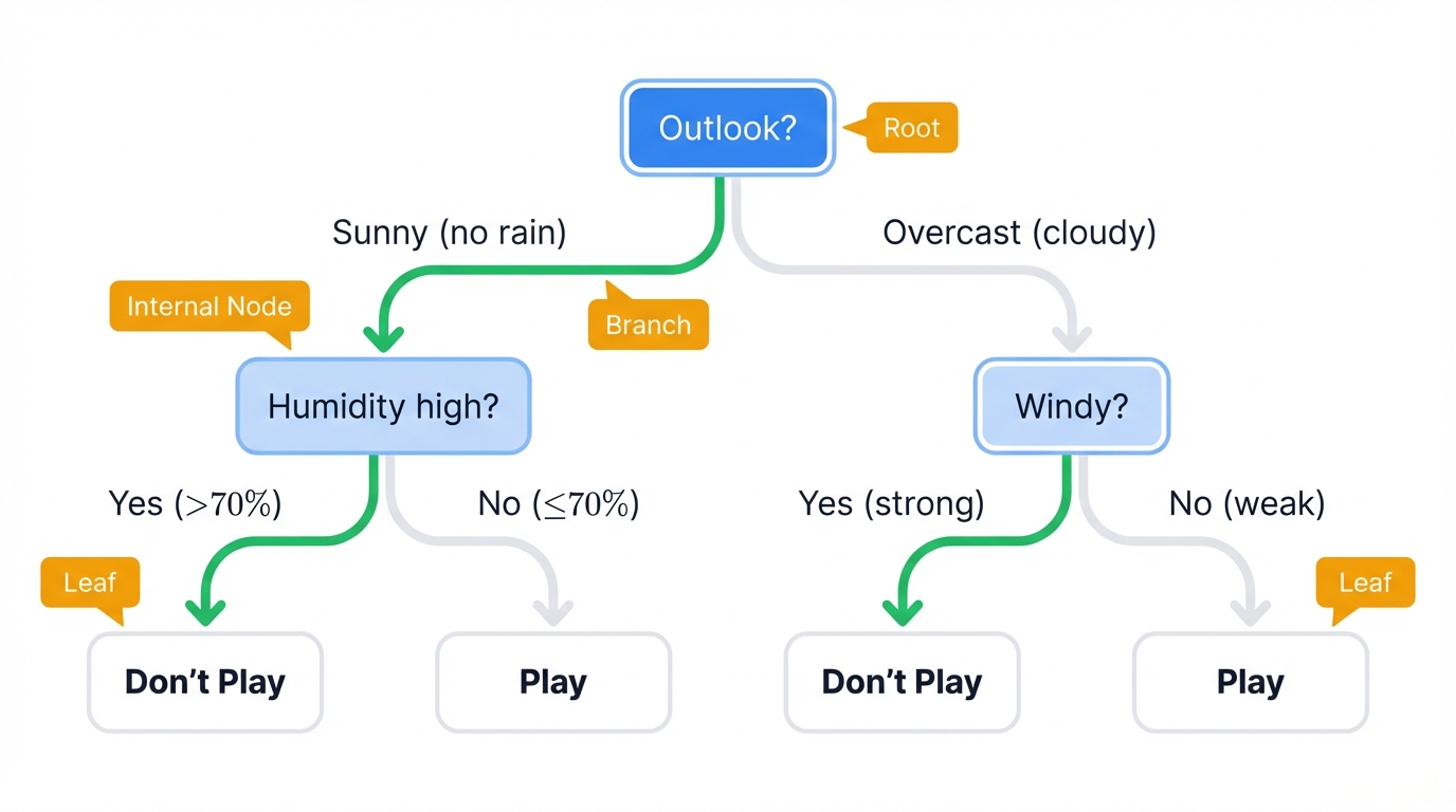
Picture an upside-down tree. It's a flowchart. These are its parts:
- Root Node: Your starting point - the entire dataset in one place
- Internal Nodes: Each asks one question about one feature: "Is age > 30?" or "Is income > $50K?"
- Branches: The yes/no paths splitting from each question
- Leaf Nodes: The final answer you came for - your prediction
Here's how it works in real life: deciding whether to play tennis. The tree asks "What's the weather outlook?" Sunny? It then asks "Is humidity high?" Yes? Prediction: "Don't Play Tennis."
This transparency makes decision trees incredibly valuable. You can trace exactly why the model made its decision - something neural networks and other "black box" methods can never give you, no matter how accurate they become, because their internal workings remain forever obscured behind layers of mathematical transformations.
Your First Decision Tree
Watch a decision tree learn. The classic "Play Tennis" dataset reveals core principles behind every tree-based model.
import numpy as np
import pandas as pd
from sklearn.tree import DecisionTreeClassifier, export_text, plot_tree
from sklearn.model_selection import train_test_split
from sklearn.metrics import accuracy_score, classification_report
import matplotlib.pyplot as plt

# Create classic "Play Tennis" dataset
data = {
    'outlook': ['sunny', 'sunny', 'overcast', 'rainy', 'rainy', 'rainy',
                'overcast', 'sunny', 'sunny', 'rainy', 'sunny', 'overcast',
                'overcast', 'rainy'],
    'temperature': ['hot', 'hot', 'hot', 'mild', 'cool', 'cool',
                    'cool', 'mild', 'cool', 'mild', 'mild', 'mild',
                    'hot', 'mild'],
    'humidity': ['high', 'high', 'high', 'high', 'normal', 'normal',
                 'normal', 'high', 'normal', 'normal', 'normal', 'high',
                 'normal', 'high'],
    'windy': [False, True, False, False, False, True,
              True, False, False, False, True, True,
              False, True],
    'play': ['no', 'no', 'yes', 'yes', 'yes', 'no',
             'yes', 'no', 'yes', 'yes', 'yes', 'yes',
             'yes', 'no']
}

df = pd.DataFrame(data)

print("Decision Tree Demo: Play Tennis Dataset")
print("=" * 40)
print("Dataset:")
print(df)
print(f"\nTarget distribution:")
print(df['play'].value_counts())

# Encode categorical variables
from sklearn.preprocessing import LabelEncoder

le_dict = {}
for column in ['outlook', 'temperature', 'humidity']:
    le = LabelEncoder()
    df[column + '_encoded'] = le.fit_transform(df[column])
    le_dict[column] = le
    print(f"\n{column.title()} encoding:")
    for i, label in enumerate(le.classes_):
        print(f"  {label}: {i}")

# Prepare features and target
feature_columns = ['outlook_encoded', 'temperature_encoded', 'humidity_encoded', 'windy']
X = df[feature_columns]
y = df['play']

print(f"\nFeatures shape: {X.shape}")
print(f"Features:")
print(X.head())

# Build decision tree
tree = DecisionTreeClassifier(
    criterion='entropy',  # Use information gain
    random_state=42,
    min_samples_split=2,  # Allow splits with as few as 2 samples
    min_samples_leaf=1    # Allow leaves with 1 sample
)

tree.fit(X, y)

# Show tree structure in text format
print(f"\nDecision Tree Rules:")
print("=" * 25)
feature_names = ['outlook', 'temperature', 'humidity', 'windy']
tree_rules = export_text(tree, feature_names=feature_names)
print(tree_rules)

# Make predictions
predictions = tree.predict(X)
accuracy = accuracy_score(y, predictions)

print(f"\nTraining Accuracy: {accuracy:.3f} ({accuracy*100:.1f}%)")
if accuracy == 1.0:
    print("🏆 Perfect fit! Tree memorized all training examples.")
    print("⚠️ This might be overfitting - would need test data to verify.")

# Test with new examples
print(f"\nTesting New Examples:")
print("-" * 25)

test_cases = [
    {'outlook': 'sunny', 'temperature': 'hot', 'humidity': 'normal', 'windy': False},
    {'outlook': 'rainy', 'temperature': 'cool', 'humidity': 'high', 'windy': True},
    {'outlook': 'overcast', 'temperature': 'mild', 'humidity': 'high', 'windy': False}
]

for i, case in enumerate(test_cases, 1):
    # Encode the test case
    encoded_case = []
    for feature in ['outlook', 'temperature', 'humidity']:
        if case[feature] in le_dict[feature].classes_:
            encoded_case.append(le_dict[feature].transform([case[feature]])[0])
        else:
            print(f"Warning: Unknown {feature} value '{case[feature]}'")
            encoded_case.append(0)  # Default to first class

    encoded_case.append(case['windy'])

    prediction = tree.predict([encoded_case])
    probability = tree.predict_proba([encoded_case])

    print(f"Case {i}: {case}")
    print(f"  Prediction: {prediction[0]}")
    print(f"  Confidence: {probability.max():.1%}")
    print()
How the tree makes decisions:
- Start at the root and check the first condition
- Follow the path based on your data (left for True, right for False)
- Continue until you hit a leaf node
- The leaf gives you the final prediction
The tree learns automatically which questions work best. It asks the most informative ones first - those that separate different outcomes most cleanly.
Random Forests: The Power of Crowds
Decision trees have one fatal flaw. They memorize training data instead of learning patterns. Random forests fix this.
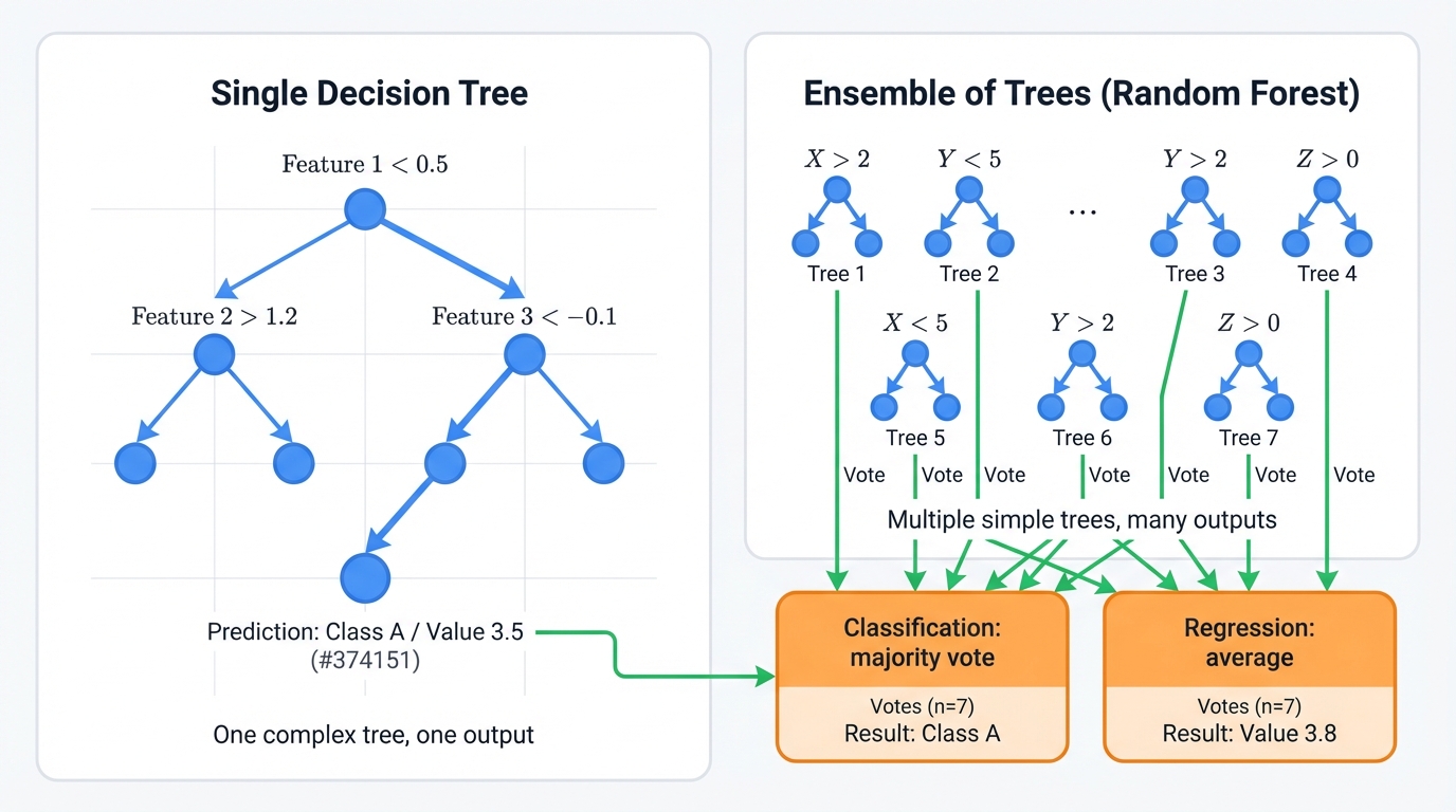
How?
Instead of trusting one tree, random forests build hundreds of slightly different trees and let them vote. Each tree trains on a random sample of your data. Each considers only random subsets of features at each split.
Making predictions works like this:
- Classification: Trees vote, majority wins
- Regression: Trees predict, algorithm averages the results
This "wisdom of crowds" approach eliminates individual tree weaknesses. A tree that overfits to noise gets outvoted by trees that learned real patterns. The result beats single trees on virtually every dataset.
The Evolution of Tree Algorithms
Decision trees didn't appear overnight. They evolved through decades of research. Each generation solved the previous version's problems. This history reveals a fundamental tension that still drives machine learning today: simple and explainable versus complex and accurate.
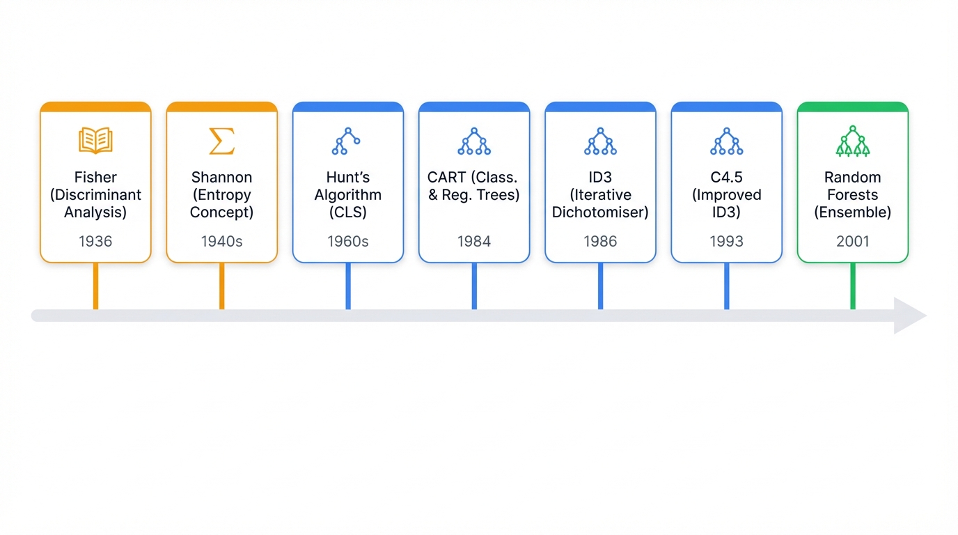
The Early Years (1930s-1960s)
Decision trees emerged from an unlikely mix. Psychology, statistics, and information theory.
Ronald Fisher's 1936 work gave us methods for classifying data into groups. Claude Shannon's information theory in the 1940s introduced entropy - a way to measure uncertainty. This became the heartbeat of tree algorithms.
The breakthrough?
Hunt's algorithm in the 1960s. Originally designed to understand how humans learn concepts, it established the top-down, recursive approach that every decision tree uses today.
The Algorithm Wars (1970s-1980s)
The 1970s and 1980s sparked a race. The goal: build the perfect decision tree. Three algorithms won. Each remains relevant today.
ID3 (1986) by Ross Quinlan was revolutionary. It introduced information gain - a systematic way to pick the best question at each split. Problems? It only worked with categorical data. It favored features with many values.
CART (1984) by Leo Breiman's team took a different approach. While ID3 asked many-way questions, CART stuck to binary splits. Yes/no questions only. It introduced Gini impurity (faster than entropy). It handled both classification and regression. CART became the foundation for modern implementations like Scikit-learn.
C4.5 (1993) fixed ID3's flaws. Quinlan added support for numerical features. Missing data handling. Gain ratio - a corrected version of information gain that didn't favor multi-valued features. C4.5 became so successful that in 2006, IEEE ranked it the top data mining algorithm.
The Ensemble Revolution (1990s-2001)
Single decision trees had a fatal flaw: they memorized training data instead of learning patterns. The solution came from an unexpected source. Crowd wisdom.
Tin Kam Ho at Bell Labs started the revolution in 1995. Random subspaces - training trees on random feature subsets. Leo Breiman added bootstrap aggregating (bagging) in 1996. Training models on random data samples.
In 2001, Breiman combined these ideas into Random Forests.
Instead of seeking one perfect tree, the approach builds many good trees and lets them vote on final predictions. This ensemble approach had three game-changing effects that transformed machine learning practice across every major industry and research domain where predictive accuracy matters more than interpretability:
- Eliminated overfitting through statistical averaging effects
- Improved accuracy across virtually every dataset type
- Traded individual tree interpretability for superior predictive performance
Machine learning shifted. From seeking the "one true model" to harnessing collective intelligence. This principle drives today's most powerful algorithms.
How Trees Learn
Decision trees and random forests use supervised learning. They need examples with known answers to learn from.
Think of teaching a child to recognize animals. Show them photos labeled "cat" or "dog" until they learn the patterns. You feed the algorithm data with features (photo characteristics) and labels (the correct animal).
The algorithm learns rules. Rules mapping features to outcomes:
- Classification: Predicting categories (spam/not spam, cat/dog/bird)
- Regression: Predicting numbers (house prices, stock returns)
Both tree types excel at both tasks.
The Math Behind the Magic
Decision trees have one obsession. Creating pure groups. "Pure" means all samples in a group have the same target value - all cats, all high-income customers, all profitable trades.
At each split, the algorithm asks: "Which question creates the biggest jump in purity?" Several mathematical measures guide this choice. The math is simpler than it looks.
Entropy and Information Gain
Entropy measures chaos in your data. High entropy equals mixed-up groups. Low entropy equals pure groups.
The formula looks intimidating. The concept is simple:
$$H(S) = -\sum_{i=1}^c p_i \log_2(p_i)$$
Where pi is the proportion of samples in class i.
Entropy Examples demonstrate how this measure captures uncertainty:
- Perfectly pure groups (all cats) achieve entropy = 0 because there's no uncertainty about class membership
- Maximum chaos scenarios (50% cats, 50% dogs) reach entropy = 1, representing maximum uncertainty where any guess is equally likely to be wrong
- Slight majority situations (70% cats, 30% dogs) produce entropy = 0.88, showing high but not maximum uncertainty
Information Gain measures how much a split reduces chaos:
Information Gain = Original Entropy - Weighted Average of Split Entropies
The algorithm picks the split with the highest information gain. The question that brings the most order to chaos.
Gain Ratio: Information Gain's Smarter Cousin
Information gain has a weakness. It loves features with many unique values. A customer ID feature with 1000 unique values will create 1000 tiny pure groups. High information gain. Useless for prediction.
Gain ratio fixes this by penalizing "cheater" features:
Gain Ratio = Information Gain / Split Info
Split Info measures how much a feature spreads out the data. Features that create many small groups get penalized. This leads to more sensible splits.
Comparing Split Criteria: Gini vs Entropy
import numpy as np
import matplotlib.pyplot as plt
from sklearn.tree import DecisionTreeClassifier
from sklearn.datasets import make_classification
from sklearn.model_selection import train_test_split
from sklearn.metrics import accuracy_score

def calculate_gini(y):
    """Calculate Gini impurity for a dataset"""
    if len(y) == 0:
        return 0

    classes, counts = np.unique(y, return_counts=True)
    probabilities = counts / len(y)
    return 1 - np.sum(probabilities ** 2)

def calculate_entropy(y):
    """Calculate entropy for a dataset"""
    if len(y) == 0:
        return 0

    classes, counts = np.unique(y, return_counts=True)
    probabilities = counts / len(y)
    # Handle log(0) case
    probabilities = probabilities[probabilities > 0]
    return -np.sum(probabilities * np.log2(probabilities))

print("Split Criteria Comparison: Gini vs Entropy")
print("=" * 42)

# Generate sample classification dataset
X, y = make_classification(
    n_samples=1000, n_features=10, n_informative=5,
    n_redundant=2, n_clusters_per_class=1, random_state=42
)

X_train, X_test, y_train, y_test = train_test_split(
    X, y, test_size=0.3, random_state=42
)

print(f"Dataset: {X.shape[0]} samples, {X.shape[1]} features")
print(f"Class distribution: {np.bincount(y)}")

# Compare Gini vs Entropy criteria
criteria = ['gini', 'entropy']
results = {}

for criterion in criteria:
    print(f"\nTraining with {criterion.title()} criterion:")

    tree = DecisionTreeClassifier(
        criterion=criterion,
        max_depth=10,
        random_state=42
    )

    tree.fit(X_train, y_train)

    # Evaluate performance
    train_accuracy = tree.score(X_train, y_train)
    test_accuracy = tree.score(X_test, y_test)

    # Tree characteristics
    n_nodes = tree.tree_.node_count
    max_depth = tree.tree_.max_depth

    results[criterion] = {
        'train_accuracy': train_accuracy,
        'test_accuracy': test_accuracy,
        'n_nodes': n_nodes,
        'max_depth': max_depth
    }

    print(f"  Training accuracy: {train_accuracy:.3f}")
    print(f"  Test accuracy: {test_accuracy:.3f}")
    print(f"  Number of nodes: {n_nodes}")
    print(f"  Maximum depth: {max_depth}")

# Compare criteria behavior with different class distributions
print(f"\n" + "="*50)
print("Impurity Measures for Different Class Distributions")
print("="*50)

class_distributions = [
    ([50, 50], "Balanced (50-50)"),
    ([80, 20], "Imbalanced (80-20)"),
    ([95, 5], "Highly imbalanced (95-5)"),
    ([100, 0], "Pure (100-0)")
]

print(f"Distribution        | Gini  | Entropy")
print("-" * 40)

for counts, description in class_distributions:
    total = sum(counts)
    y_sample = np.repeat([0, 1], counts) if counts[1] > 0 else np.repeat([0], [total])

    gini = calculate_gini(y_sample)
    entropy = calculate_entropy(y_sample)

    print(f"{description:18s} | {gini:6.3f} | {entropy:7.3f}")

print(f"\nKey Insights:")
print(f"1. Both reach 0 for pure nodes (perfect classification)")
print(f"2. Both peak at balanced distributions")
print(f"3. Gini is faster to compute (no logarithms)")
print(f"4. Entropy is more sensitive to probability changes")
print(f"5. In practice, performance differences are usually small")

# Demonstrate Information Gain calculation
print(f"\n" + "="*40)
print("Information Gain Example")
print("="*40)

# Simple example: Splitting on a binary feature
y_before = np.array([0, 0, 0, 1, 1, 1, 1, 1])  # 3 zeros, 5 ones
feature = np.array([0, 0, 1, 0, 1, 1, 1, 1])   # Binary feature

print(f"Before split: {y_before}")
print(f"Feature values: {feature}")

# Calculate initial entropy
initial_entropy = calculate_entropy(y_before)
print(f"\nInitial entropy: {initial_entropy:.3f}")

# Split based on feature
left_indices = feature == 0
right_indices = feature == 1

y_left = y_before[left_indices]
y_right = y_before[right_indices]

print(f"\nAfter split:")
print(f"Left (feature=0): {y_left}")
print(f"Right (feature=1): {y_right}")

# Calculate entropy after split
entropy_left = calculate_entropy(y_left)
entropy_right = calculate_entropy(y_right)

print(f"\nEntropy left: {entropy_left:.3f}")
print(f"Entropy right: {entropy_right:.3f}")

# Weighted average entropy after split
weight_left = len(y_left) / len(y_before)
weight_right = len(y_right) / len(y_before)
weighted_entropy = weight_left * entropy_left + weight_right * entropy_right

# Information gain
information_gain = initial_entropy - weighted_entropy

print(f"\nWeighted entropy after split: {weighted_entropy:.3f}")
print(f"Information Gain: {information_gain:.3f}")

if information_gain > 0:
    print("✓ Good split! Reduced uncertainty.")
else:
    print("✗ Poor split! No improvement in purity.")
Visualizing the Difference
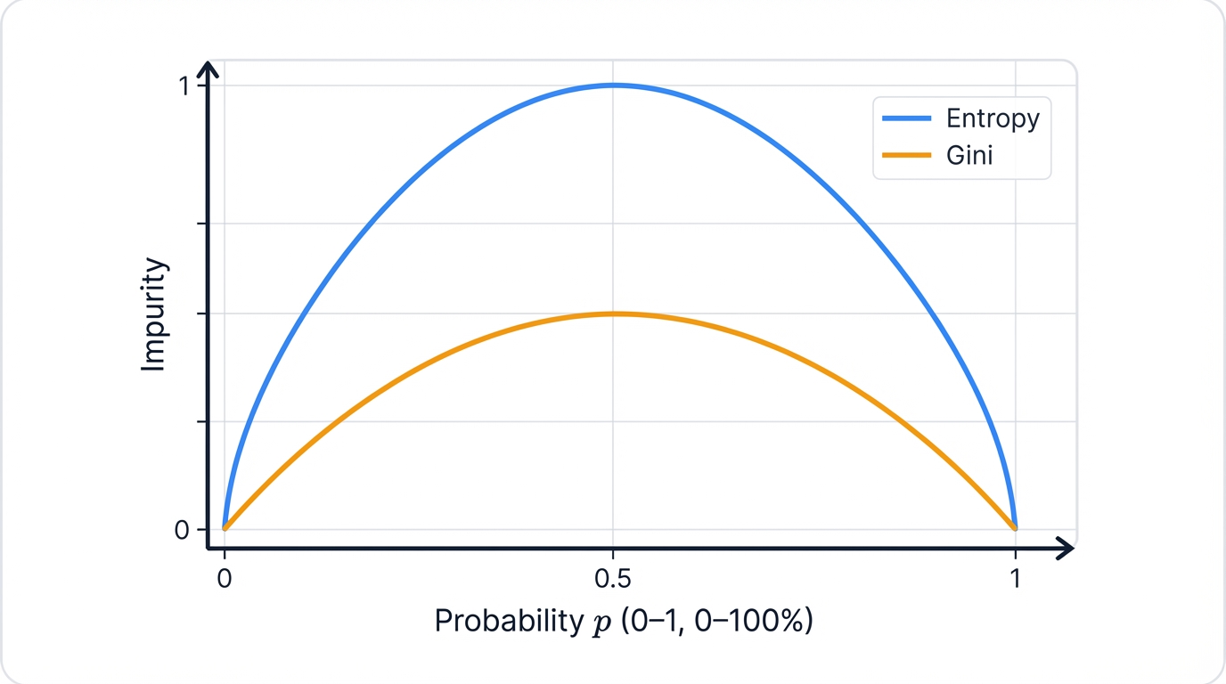
Gini vs Entropy Behavior:
 Impurity ↑
     1.0 │ ┌────────────┐ ← Entropy (curved)
         │ ╭              ╮
     0.5 │╭                ╮ ← Gini (parabolic)
         ╱                  ╲
     0.0 │────────────────────────→
        0%   25%   50%   75%   100%
            Proportion of Class 1
Key insights:
- Both metrics hit zero at pure splits where all samples belong to the same class (0% or 100% purity)
- Both peak at 50-50 splits where uncertainty reaches maximum levels with equal class distribution
- Entropy is more sensitive to changes in class distribution, making it better at detecting subtle improvements in purity
- Gini is faster to calculate. Simpler math. Preferred for large datasets where computational efficiency matters.
- Performance differences are minimal in practice, so the choice comes down to computational considerations rather than accuracy gains
Gini Impurity: The Faster Alternative
Gini impurity asks a simple question. "If I randomly pick a sample and randomly guess its class, what's the probability I'm wrong?"
$$\text{Gini}(S) = 1 - \sum_{i=1}^c p_i^2$$
Where pi is the proportion of samples in class i.
Gini Examples illustrate how this measure captures the probability of misclassification:
- Pure groups (all cats) achieve Gini = 0 because random guessing cannot be wrong when only one class is present
- 50/50 splits reach Gini = 0.5, representing maximum uncertainty where random guessing is wrong half the time
- Heavily skewed distributions (90% cats, 10% dogs) produce Gini = 0.18, indicating low uncertainty due to strong class imbalance
Gini vs Entropy Trade-offs:
- Speed advantages favor Gini. It avoids logarithmic calculations that entropy requires.
- Behavioral differences show Gini favoring isolation of majority classes while Entropy creates more balanced splits
- Performance outcomes are identical in practice. Computational efficiency becomes the primary selection criterion.
Most implementations (including Scikit-learn) default to Gini. Speed wins.
Variance Reduction: For Continuous Targets
Regression trees can't use Gini or entropy. They need a way to measure "closeness" of continuous values.
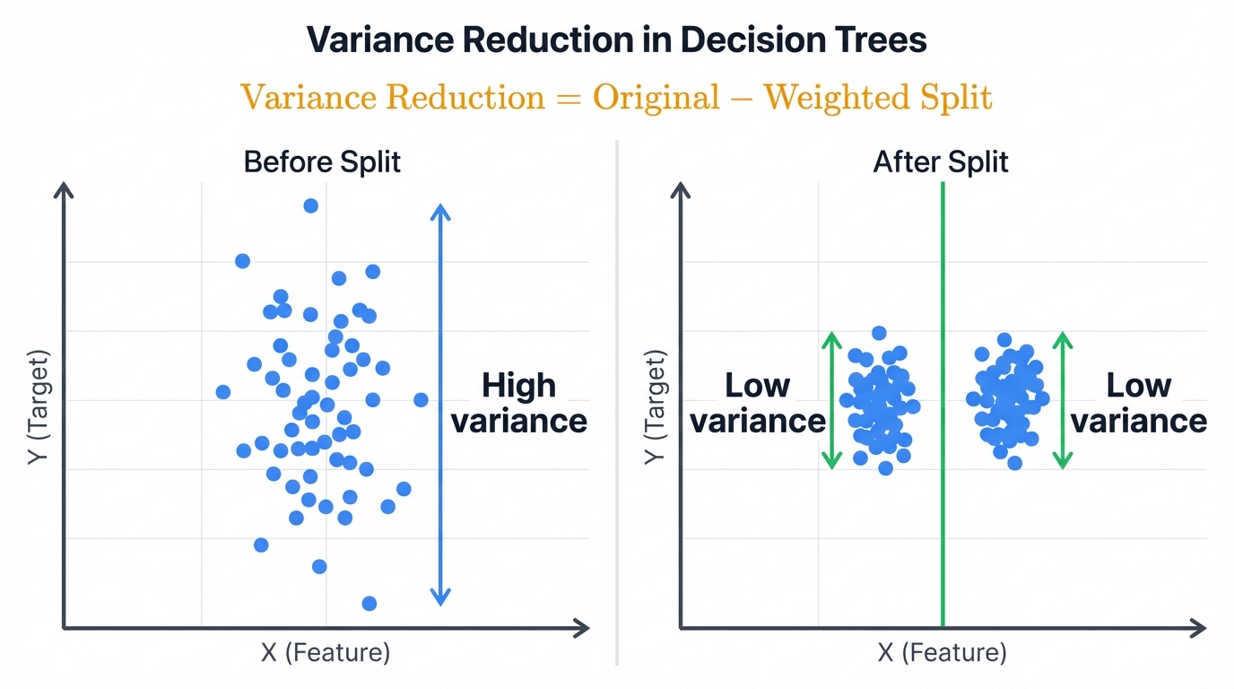
Variance becomes the impurity measure. High variance equals values spread out. Low variance equals values clustered together.
Variance Reduction = Original Variance - Weighted Average of Split Variances
The algorithm picks splits that create groups with similar target values. Most implementations use Mean Squared Error (MSE). Mathematically equivalent. Computationally simpler.
Note: This comprehensive guide continues with extensive coverage of Random Forest implementations, ensemble methods, production deployment strategies, hyperparameter tuning, interpretability techniques, scalability considerations, and advanced variants. The complete article represents one of the most thorough treatments of decision trees and random forests available, spanning from foundational theory through practical implementation to cutting-edge research developments.